Internals of the film-loop program

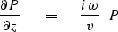
The differential equation solved by the program is equation (5), copied here as  

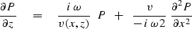$${\partial P \over \partial z } \eq { i \, \omega \over v(x,... ...er - \, i \, \omega \, 2 } \ {\partial^2 P \over \partial x^2}$$ (43)

For each $\Delta\,z$-step the calculation is done in two stages. The first stage is to solve  

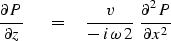$${\partial P \over \partial z} \ \eq {v \over - \, i \, \omega \, 2} \ {\partial^2 P \over \partial x^2}$$ (44)

Using the Crank-Nicolson differencing method this becomes

$${ p_{{z+1}}^x - p_z^x \over \Delta z } \eq {v \over -i\omega... ...p_{{z+1}}^x + p_{{z+1}}^{{x-1}} \over 2\, \Delta x^2 } \right)$$ (45)

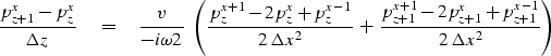
Absorb all the constants into one and define  

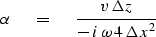$$\alpha \ \eq \ {v \, \Delta z \over -\,i\,\omega\,4\, \Delta x^2 }$$ (46)

getting

$$p_{{z+1}}^x \,-\, p_z^x \eq \alpha \, \left[ \, ( \, p_z^{{x... ...+1}}\,-\, 2 \, p_{{z+1}}^x \,+\, p_{{z+1}}^{{x-1}} ) \, \right]$$ (47)

Bring the unknowns to the left:  

$$- \alpha p_{{z+1}}^{{x+1}} \,+\, ( 1+2 \alpha ) p_{{z+1}}^x ... ...p_z^{{x+1}} \,+\, (1-2 \alpha ) p_z^x \,+\, \alpha p_z^{{x-1}}$$ (48)

We will solve this as we solved equations (32) and (33). The second stage is to solve the equation  

$${\partial P \over \partial z} \ \eq \ {i\,\omega \over v }\ \ P$$ (49)

analytically by  

$$P(z+ \Delta z) \ \eq \ P(z) \ e^{i \Delta z \ \omega / v }$$ (50)

By alternating between (48) and (50), which are derived from (44) and (49), the program solves (43) by a splitting method. The program uses the tridiagonal solver discussed earlier, like subroutine rtris() except that version needed here, ctris(), has all the real variables declared complex.

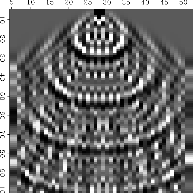
Figure 4 shows a change of initial conditions where the incoming wave on the top frame is defined to be an impulse, namely, p(x,z=0) = $(\cdots,0,0,1,0,0,\cdots)$.The result is alarmingly noisy. What is happening is that for any frequencies anywhere near the Nyquist frequency, the difference equation departs from the differential equation that it should mimic. This problem is addressed, analyzed, and ameliorated in IEI. For now, the best thing to do is to avoid sharp corners in the initial wave field.

 

Mcompart90 Figure 4 Observe and describe various computational artifacts by testing the program using a point source at (x,z) = (xmax/2,0). Such a source is rich in the high spatial frequencies for which difference equations do not mimic their differential counterparts. (Movie)