


Another important application of the algebra associated with Toeplitz matrices is in high-resolution spectral analysis. This is where a power spectrum is to be estimated from a sample of data which is short (in time or space). The conventional statistical and engineering knowledge in this subject is based on assumptions which are frequently inappropriate in geophysics. The situation was fully recognized by John P. Burg who utilized some of the special properties of Toeplitz matrices to develop his maximum-entropy spectral estimation procedure described in a later chapter.
Another place where Toeplitz matrices play a key role is in the mathematical physics which describes layered materials. Geophysicists often model the earth by a stack of plane layers or by concentric spherical shells where each shell or layer is homogeneous. Surprisingly enough, many mathematical physics books do not mention Toeplitz matrices. This is because they are preoccupied with forward problems; that is, they wish to calculate the waves (or potentials) observed in a known configuration of materials. In geophysics, we are interested in both forward problems and in inverse problems where we observe waves on the surface of the earth and we wish to deduce material configurations inside the earth. A later chapter contains a description of how Toeplitz matrices play a central role in such inverse problems.
We start with a time function xt which may or may not be minimum phase.
Its spectrum is computed by ![]() .As we saw in the preceding sections,
given R(Z) alone there is no way of knowing whether
it was computed from a minimum-phase function or a nonminimum-phase function.
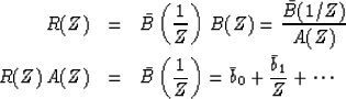
We may suppose that there exists a minimum phase B(Z) of the given spectrum,
that is,
.As we saw in the preceding sections,
given R(Z) alone there is no way of knowing whether
it was computed from a minimum-phase function or a nonminimum-phase function.
We may suppose that there exists a minimum phase B(Z) of the given spectrum,
that is, ![]() .Since B(Z) is by hypothesis minimum phase,
it has an inverse A(Z) = 1/B(Z).
We can solve for the inverse A(Z) in the following way:
.Since B(Z) is by hypothesis minimum phase,
it has an inverse A(Z) = 1/B(Z).
We can solve for the inverse A(Z) in the following way:
 |
(7) | |
| (8) |
| |
(9) |
| r1 a0 + r0 a1 + r-1 a2 = 0 | (10) |
| r2 a0 + r1 a1 + r0 a2 = 0 | (11) |
![\begin{displaymath}
\left[
\begin{array}
{lll}
r_0 & r_{-1} & r_{-2} \\ r_1 & ...
...ft[
\begin{array}
{c}
\bar b_0 \\ 0 \\ 0 \end{array} \right]\end{displaymath}](img37.gif) |
(12) |
![\begin{displaymath}
\left[
\begin{array}
{lll}
r_0 & r_{-1} & r_{-2} \\ r_1 & ...
...\eq \left[
\begin{array}
{c}
v \\ 0 \\ 0 \end{array} \right]\end{displaymath}](img40.gif) |
(13) |
At this point, a pessimist might interject that the polynomial A(Z) = a0 + a1 Z + a2 Z2 determined from solving the set of simultaneous equations might not turn out to be minimum phase, so that we could not necessarily compute B(Z) by B(Z) = 1/A(Z). The pessimist might argue that the difficulty would be especially likely to occur if the size of the set (13) was not taken to be large enough. Actually experimentalists have known for a long time that the pessimists were wrong. A proof can now be performed rather easily, along with a description of a computer algorithm which may be used to solve (13).
The standard computer algorithms for solving simultaneous equations require time proportional to n3 and computer memory proportional to n2. The Levinson computer algorithm for Toeplitz matrices requires time proportional to n2 and memory proportional to n. First notice that the Toeplitz matrix contains many identical elements. Levinson utilized this special Toeplitz symmetry to develop his fast method.
The method proceeds by the approach called recursion.
That is, given the solution to the ![]() set of equations,
we show how to calculate the solution to the
set of equations,
we show how to calculate the solution to the ![]() set.
One must first get the solution for k = 1;
then one repeatedly (recursively) applies a set of formulas
increasing k by one at each stage.
We will show how the recursion works for real-time functions
(rk = r-k) going from the
set.
One must first get the solution for k = 1;
then one repeatedly (recursively) applies a set of formulas
increasing k by one at each stage.
We will show how the recursion works for real-time functions
(rk = r-k) going from the ![]() set of equations
to the
set of equations
to the ![]() set, and leave it to the reader
to work out the general case.
set, and leave it to the reader
to work out the general case.
Given the ![]() simultaneous equations and their solution a1
simultaneous equations and their solution a1
![\begin{displaymath}
\left[
\begin{array}
{lll}
r_0 & r_{1} & r_{2} \\ r_1 & r_...
...\eq \left[
\begin{array}
{c}
v \\ 0 \\ 0 \end{array} \right]\end{displaymath}](img46.gif) |
(14) |
![\begin{displaymath}
\left[
\begin{array}
{llll}
r_0 & r_{1} & r_{2} & r_3 \\ r...
...left[
\begin{array}
{c}
v \\ 0 \\ 0 \\ e\end{array} \right]\end{displaymath}](img47.gif) |
(15) |
![\begin{displaymath}
\left[
\begin{array}
{llll}
r_0 & r_{1} & r_{2} & r_3 \\ r...
...eft[
\begin{array}
{c}
v' \\ 0 \\ 0 \\ 0\end{array} \right]\end{displaymath}](img48.gif) |
(16) |
The important trick is that from (15) one can write a ``reversed'' system of equations. (If you have trouble with the matrix manipulation, merely write out (16) as simultaneous equations, then reverse the order of the unknowns, and then reverse the order of the equations.)
![\begin{displaymath}
\left[
\begin{array}
{llll}
r_0 & r_{1} & r_{2} & r_3 \\ r...
...left[
\begin{array}
{c}
e \\ 0 \\ 0 \\ v\end{array} \right]\end{displaymath}](img49.gif) |
(17) |
![\begin{displaymath}
\left[
\begin{array}
{llll}
r_0 & r_{1} & r_{2} & r_3 \\ r...
...egin{array}
{c}
e \\ 0 \\ 0 \\ v\end{array} \right] \right\}\end{displaymath}](img50.gif) |
(18) |
![\begin{eqnarray}
e &\leftarrow & \sum^2_{i = 0} a_i r_{3 - i}
\\ \left[ \begin{a...
...a_1 \\ 1\end{array} \right]
\\ v' &\leftarrow & v\, [1 - (e/v)^2]\end{eqnarray}](img51.gif) |
(19) | |
| (20) | ||
| (21) |
We have shown how to calculate the solution of the ![]() Toeplitz
equations from the solution of the
Toeplitz
equations from the solution of the ![]() Toeplitz equations.
The Levinson recursion consists of doing this type of step,
starting from
Toeplitz equations.
The Levinson recursion consists of doing this type of step,
starting from ![]() and working up to
and working up to ![]() .
.
       COMPLEX R,A,C,E,BOT,CONJG
       C(1)=-1.; R(1)=1.; A(1)=1.; V(1)=1.
  200  DO 220 J=2,N
       A(J)=0.
       E=0.
       DO 210 I=2,J
  210  E=E+R(I)*A(J-I+1)
       C(J)=E/V(J-1)
       V(J)=V(J-1)-E*CONJG(C(J))
       JH=(J+1)/2
       DO 220 I=1,JH
       BOT=A(J-I+1)-C(J)*CONJG(A(I))
       A(I)=A(I)-C(J)*CONJG(A(J-I+1))
  220  A(J-I+1)=BOT

Let us reexamine the calculation
to see why A(Z) turns out to be minimum phase.
First, we notice that
![]() and
and ![]() are always positive.
Then from (21) we see that
-1 < e/v < +1.
(The fact that c = e/v is bounded by unity will later be shown
to correspond to the fact that reflection coefficients for waves are so
bounded.)
Next, (20) may be written in polynomial form as
are always positive.
Then from (21) we see that
-1 < e/v < +1.
(The fact that c = e/v is bounded by unity will later be shown
to correspond to the fact that reflection coefficients for waves are so
bounded.)
Next, (20) may be written in polynomial form as
| |
(22) |
1. R(Z) is of the form ![]() .
.
2. |ck| < 1.
3. A(Z) is minimum phase.
If any one of the above three is false, then they are all false. A program for the calculation of ak and ck from rk is given in Figure 3. In Chapter 8, on wave propagation in layers, programs are given to compute rk from ak or ck.
![]()
![]()
Toeplitz matrices are found in the mathematical literature under the topic of polynomials orthogonal on the unit circle. The author especially recommends Atkinson's book.