


In recent years, a popular view of geophysical data modeling has been that the earth is a continuum and that we should regard the number of unknowns as infinite but the number of our observations as finite. In a computer one therefore approximates the situation by a highly underdetermined system of simultaneous equations. In order to get a unique answer, the solution should extremalize some integral. In practice, a sum of squares is often minimized in such a way as to produce a smooth solution. A typical mathematical formulation is to do a least squares fitting of an equation set like
| (61) |
where the top of block ![]() denotes the underdetermined constraint equations
with the data vector
denotes the underdetermined constraint equations
with the data vector ![]() ;the unknowns are in the
;the unknowns are in the ![]() vector;
and the bottom block is a band matrix
(all the nonzero elements cluster about the diagonal)
which says that some filtered version of
vector;
and the bottom block is a band matrix
(all the nonzero elements cluster about the diagonal)
which says that some filtered version of ![]() should vanish.
The filter is often a roughing filter
like the first-difference operator.
In the absence of data,
the first-difference operator
leads to a constant solution which is sensible.
What is not sensible is that
it forces the result to be smoothed
even though realistic earth models often
contain step discontinuities
(where two homogeneous media lie in contact).
should vanish.
The filter is often a roughing filter
like the first-difference operator.
In the absence of data,
the first-difference operator
leads to a constant solution which is sensible.
What is not sensible is that
it forces the result to be smoothed
even though realistic earth models often
contain step discontinuities
(where two homogeneous media lie in contact).
The choice of a filter is a rather subjective matter, the choice often being made on the basis of the solution it will produce. Unfortunately, the solution is often a rather sensitive function of the subjectively chosen weights and filters; this fact makes the whole business an art, a matter of experience and judgment. General purpose theories of inversion exist, but they do not prepare the geophysicist to exploit the peculiarities of any particular situation or data set. Inversion theories, like mathematical statistics, should be used like a lamp post - to light the way, not to lean upon.
One useful concept in inversion theory is the idea of coordinate-system invariance. The idea is that one should get the same answer in an electrical conductivity problem whether one parameterizes the earth by an unknown conductivity at every point on a sufficiently dense mesh, or one parameterizes with resistivity on the mesh, or one parameterizes by coefficients of some expansion in a complete set of basis functions. Clearly, the idea of fitting low-order coefficients in some expansion setting the high-order coefficients equal to zero is not a coordinate-invariant approach. A different origin for polynomial expansions can change everything. A different set of basis functions would change everything. Of course, it is not essential to use a coordinate-system invariant technique in data inversion. But if one does not, one should beware of the sensitivity of one's solution to changes in the coordinate system.
|
6-2
Figure 1 Minimizing either of these two functions will drive p toward | 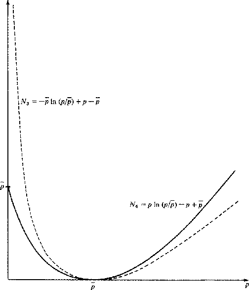 |

Let us consider some inversion procedures
which are coordinate-system invariant.
We will restrict ourselves to physical problems
in which we can identify a positive density function p
as energy or dissipation per unit volume.
Let us denote by ![]() the value of this power
as a function of space
in the default model of the earth.
The default model is the one we want to find
when we have no measurements.
It will often be one in which
the material properties are constant functions of space.
Now we will need some functions
which we will call model norms.
They have the properties of being positive
for all (positive) p and
the value of this power
as a function of space
in the default model of the earth.
The default model is the one we want to find
when we have no measurements.
It will often be one in which
the material properties are constant functions of space.
Now we will need some functions
which we will call model norms.
They have the properties of being positive
for all (positive) p and ![]() and
being minimized at
and
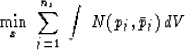
being minimized at ![]() .Some examples plotted in Figure 1 are
.Some examples plotted in Figure 1 are
 |
||
Now let the adjustable earth properties be denoted by x,
a function of space.
We can choose x to minimize some volume integral
of one of the model norms
subject to the constraint that the model produce the
required observations.
Sometimes we have observations from
![]() source locations.
We then need to compute the default power
distribution
source locations.
We then need to compute the default power
distribution ![]() for each.
Then we can minimize a sum of volume integrals
for each.
Then we can minimize a sum of volume integrals
It will be noted that the model-norm functions
are all homogeneous of order 1.
This means that ![]() for a > 0.
This is our assurance that
N is a volume density.
Without this property
we would have the difficulty that a sum of
for a > 0.
This is our assurance that
N is a volume density.
Without this property
we would have the difficulty that a sum of
![]() over a set of subvolumes
over a set of subvolumes
![]() would change as the mesh were refined.
Coordinate-system invariance is provided by the usual rules
for conversion of volume integrals from one coordinate system to another.
would change as the mesh were refined.
Coordinate-system invariance is provided by the usual rules
for conversion of volume integrals from one coordinate system to another.
Now let us take up an example from filter theory
which turns out to be related to maximum-entropy spectral estimation.
We are given a known input spectrum R(Z)
and are to find the finite length filter
![]() whose output is as white as possible in the sense of
minimizing the integral of N3 across the spectrum.
Let the spectrum of the filter
be
whose output is as white as possible in the sense of
minimizing the integral of N3 across the spectrum.
Let the spectrum of the filter
be ![]() .We have
.We have ![]() and
and ![]() .Thus, the minimization is
.Thus, the minimization is
![]()
![\begin{eqnarray}
0 &=& \int \, \left( - {1 \over S} + R \right)
\, {\partial S ...
... - {1 \over \bar{X}(1/Z)} + R(Z)X(Z) \right]
\, d\omega \nonumber\end{eqnarray}](img172.gif) |
||
Since we know that minimum-phase functions
can represent any spectrum,
we take ![]() to be expandable as
to be expandable as ![]()
![]()
We recall that this integral selects the coefficient
of Z0 of the argument.
If we suppose that the filter is constrained to have
xk = 0 for ![]() ,we get the familiar Toeplitz system
,we get the familiar Toeplitz system
![\begin{displaymath}
\left[
\begin{array}
{ccc}
r_0 & r_{-1} & r_{-2} \\ r_1 &...
...q \left[
\begin{array}
{c}
b_0 \\ 0 \\ 0 \end{array} \right]\end{displaymath}](img177.gif)