INVERSE LINEAR INTERPOLATION

In Chapter we defined linear interpolation

as the extraction of values from between mesh points. In a typical setup (occasionally the role of data and model are swapped), a model is given on a uniform mesh and we solve the easy problem of extracting values between the mesh points with subroutine lint1() . The genuine problem is the inverse problem, which we attack here. Data values are sprinkled all around, and we wish to find a function on a uniform mesh from which we can extract that data by linear interpolation. The adjoint operator for subroutine lint1() simply piles data back into its proper location in model space without regard to how many data values land in each region. Thus some model values may have many data points added to them while other model values get none. We could interpolate by minimizing the energy in the gradient, or that in the second derivative of the model, or that in the output of any other roughening filter applied to the model.

Formalizing now our wish that data $\bold d$ be extractable by linear interpolation $\bold L$,from a model $\bold m$,and our wish that application of a roughening filter with an operator $\bold A$ have minimum energy, we write the fitting goals:  

$$\begin{array} {lll} \bold 0 &\approx & \bold L \bold m - \bold d \\ \bold 0 &\approx & \bold A \bold m \end{array}$$ (20)

Suppose we take the roughening filter to be the second difference operator (1,-2,1) scaled by a constant $\epsilon$,and suppose we have a data point near each end of the model and a third data point exactly in the middle. Then, for a model space 7 points long, the fitting goal could look like

 

$${ \left[ \begin{array} {rrrrrr} .8 & .2 & . & . & . & . \... ... \bold r_m \end{array} \right] \quad \approx \ \bold 0 }$$ (21)

The residual vector has two parts, a data part $\bold r_d$ on top and a model part $\bold r_m$ on the bottom. The data residual should vanish except where contradictory data values happen to lie in the same place. The model residual is the roughened model.

Two fitting goals (20) are so common in practice that it is convenient to adopt our least-square fitting subroutine solver accordingly. The modification is shown in module reg_solver . In addition to specifying the ``data fitting'' operator $\bold L$(parameter oper), we need to pass the ``model regularization'' operator $\bold A$(parameter reg) and the size of its output (parameter nreg) for proper memory allocation. (When I first looked at module reg_solver I was appalled by the many lines of code, especially all the declarations. Then I realized how much much worse was Fortran 77 where I needed to write a new solver for every pair of operators. This one solver module works for all operator pairs and for many optimization descent strategies because these ``objects'' are arguments. These objects require declarations that are more complicated than the simple objects of Fortran 77.)

 

module reg_solver  {
  logical, parameter, private  :: T = .true., F = .false.
contains
  subroutine solver_reg( oper, solv, reg, nreg, x, dat, niter, eps, x0)  {
    optional                                                     :: x0   
    interface {
       integer function oper(  adj, add, x, dat) {
            logical, intent( in) :: adj, add
            real, dimension( :)  :: x, dat
            }
       integer function reg(   adj, add, x, dat) {
            logical, intent( in) :: adj, add
            real, dimension( :)  :: x, dat
            }
       integer function solv(  forget, x, g, rr, gg) {
            logical             :: forget
            real, dimension( :) :: x, g, rr, gg
            }
       }
    real, dimension( :), intent( in)  :: dat, x0          # data, initial
    real, dimension( :), intent( out) :: x                # solution
    real,                intent( in)  :: eps              # scaling
    integer,             intent( in)  :: niter, nreg      # iterations, size 
    real, dimension( size( x))        :: g                # gradient
    real, dimension( size( dat) + nreg), target :: rr, gg # residual, conj grad
    real, dimension( :), pointer      :: rd,rm,gd,gm
    integer                           :: i, stat1, stat2, stat
    rm => rr( 1: nreg); rd => rr( 1 + nreg:)          # model and data resids
    gm => gg( 1: nreg); gd => gg( 1 + nreg:)          # model and data grads
                        rd = - dat                    # initialize r_d
    if( present( x0)) {
       stat1 = oper( F, T, x0, rd)    # r_d = L x0 - dat  
       stat2 =  reg( F, F, x0, rm)    # r_m = eps A x0 
                          rm = rm*eps #
                          x = x0          }             # start with x0
    else {                x = 0.;  rm = 0.}             # start with zero
    do i = 1, niter  {
       stat1 = oper( T, F, g, rd)     # g   = L' r_d
	                 gm = rm*eps  #   
       stat2 =  reg( T, T, g, gm)     # g   = L' r_d + eps A' r_m
       stat1 = oper( F, F, g, gd)     # g_d = L g
       stat2 =  reg( F, F, g, gm)     # g_m = eps A g
                         gm = gm*eps  #
       stat  = solv( F, x, g, rr, gg) # step in x and rr
       }
  }
}

First we load the data part of the residual $\bold r_d=\bold L \bold m_0 - \bold d$and the model part of the residual $\bold r_m = \bold A \bold m_0$.After the initialization, the subroutine invint1() begins an iteration loop by first computing the proposed model perturbation $\Delta \bold m$with the adjoint operator:

$$\Delta \bold m \quad\longleftarrow\quad \left[ \begin{arr... ...\begin{array} {c} \bold r_d \\ \bold r_m \end{array} \right]$$ (22)

Using this value of $\Delta \bold m$,we can find the implied change in residual $\Delta\bold r$ as

$$\Delta \left[ \begin{array} {c} \bold r_d \\ \bold r_m ... ...c} \bold L \\ \bold A \end{array} \right] \ \Delta \bold m$$ (23)

and the last thing in the loop is to use the optimization step function solv() to choose the length of the step size and to choose how much of the previous step to include.

An example of using the new solver is subroutine invint1 I chose to implement the model roughening operator $\bold A$with the convolution subroutine tcai1() , which has transient end effects (and an output length equal to the input length plus the filter length). The adjoint of subroutine tcai1() suggests perturbations in the convolution input (not the filter).  

module invint {                      # invint - INVerse INTerpolation in 1-D.
  use lint1
  use tcai1
  use cgstep_mod
  use reg_solver
contains
  subroutine invint1( niter, coord, dd, o1, d1, aa, mm, eps) {
    integer,               intent (in)   :: niter               # iterations
    real,                  intent (in)   :: o1, d1, eps         # axis, scale
    real, dimension (:),   pointer       :: coord, aa           # aa is filter
    real, dimension (:),   intent (in)   :: dd                  # data
    real, dimension (:),   intent (out)  :: mm                  # model
    integer                              :: nreg                # size of A m
    nreg = size( aa) + size( mm)                                # transient

call lint1_init( o1, d1, coord )                            # interpolation
    call tcai1_init( aa, size( mm))                             # filtering

call solver_reg( lint1_lop, cgstep, tcai1_lop, nreg, mm, dd, niter, eps)
    call cgstep_close( )
    }
}

Figure 11 shows an example for a (1,-2,1) filter with $\epsilon = 1$.The continuous curve representing the model $\bold m$passes through the data points. Because the models are computed with transient convolution end-effects, the models tend to damp linearly to zero outside the region where signal samples are given.

 

im1-2+190 Figure 11 Sample points and estimation of a continuous function through them.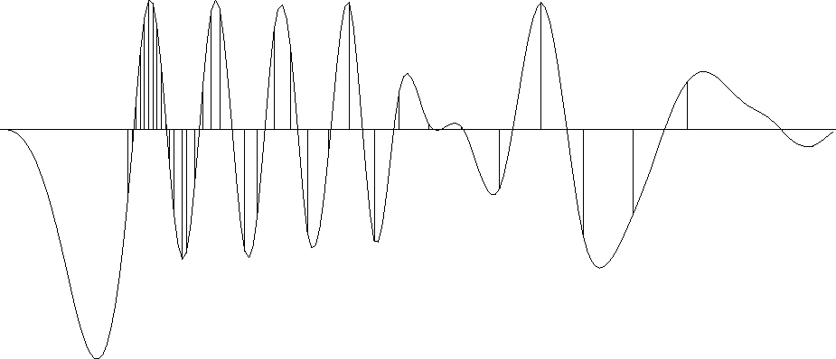

To show an example where the result is clearly a theoretical answer, I prepared another figure with the simpler filter (1,-1). When we minimize energy in the first derivative of the waveform, the residual distributes itself uniformly between data points so the solution there is a straight line. Theoretically it should be a straight line because a straight line has a vanishing second derivative, and that condition arises by differentiating by $\bold x'$,the minimized quadratic form $\bold x' \bold A' \bold A \bold x$, and getting $\bold A' \bold A \bold x=\bold 0$.(By this logic, the curves between data points in Figure 11 must be cubics.) The (1,-1) result is shown in Figure 12.

 

im1-1a90 Figure 12 The same data samples and a function through them that minimizes the energy in the first derivative.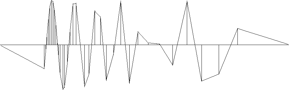