Interlacing a filter

The filter below, however, can be designed despite alternate missing traces, because it can destroy plane waves. If the plane wave should happen to pass halfway between the ``d'' and the ``e'', those two points could interpolate the halfway point, at least for well-sampled temporal frequencies, and the time axis should always be well sampled.  

$$\begin{array} {ccccccccc} a &\cdot &b &\cdot &c &\cdot &d &... ...&\cdot &\cdot &\cdot &1 &\cdot &\cdot &\cdot &\cdot \end{array}$$ (1)

We could use module pef to find the filter (1), if we set up the lag table lag appropriately. Then we could throw away alternate zeroed rows and columns (rescale the lag) to get the filter  

$$\begin{array} {ccccc} a &b &c &d &e \\ \cdot &\cdot &1 &\cdot &\cdot \end{array}$$ (2)

which could be given to subroutine mis1() , because both the filters (1) and (2) have the same dip characteristics.  

module lace {                               # interlace missing traces
  use boundary
  use pef
  use format
  use mis2
contains
  subroutine interlace( dd, xx, known, niter, j, n1,n2, lag1,lag2, a1,a2,a3) {
    integer, intent( in)            :: niter, j, n1,n2, lag1,lag2, a1,a2,a3
    real,    dimension (:)          :: xx                     # output
    logical, dimension (:), pointer :: known, bad             # selectors
    real,    dimension (:), pointer :: dd, aa                 # input, PEF
    integer, dimension (:), pointer :: small, large           # helix lags
    integer                         :: i1, i2, i3, na, i
    na = (a1-lag1) + (a2-lag2)*a1 + (a3-1)*a1*a2              # filter size
    allocate (small (na), large (na), aa (na), bad(size(dd)))
    do i3 = 1, a3 {                                           # find helix lags
    do i2 = 1, a2 { if( i3 == 1 .and. i2 < lag2                  ) cycle
    do i1 = 1, a1 { if( i3 == 1 .and. i2 == lag2 .and. i1 <= lag1) cycle
	      i  =  i1-lag1    + (i2-lag2)*a1 + (i3-1)*a1*a2
       small( i) =  i1-lag1    + (i2-lag2)*n1 + (i3-1)*n1*n2  # a(i1,i2,i3)
       large( i) = (i1-lag1)*j + (i2-lag2)*n1 + (i3-1)*n1*n2  # j = jump
    }}}
    call bound3 (n1,n2,lag1*j,lag2,a1*j,a2,a3,bad)            # bad regressors
    call find_pef  (dd, aa, large, bad, na*2)                 # estimate aa
    call print3 (n1,n2,lag1,  lag2,a1,  a2,a3,aa, small)      # print aa
    call mis1 (niter, xx, aa, small, known, .false., .false.) # interlace
    deallocate (small, large, aa, bad)
  }
}

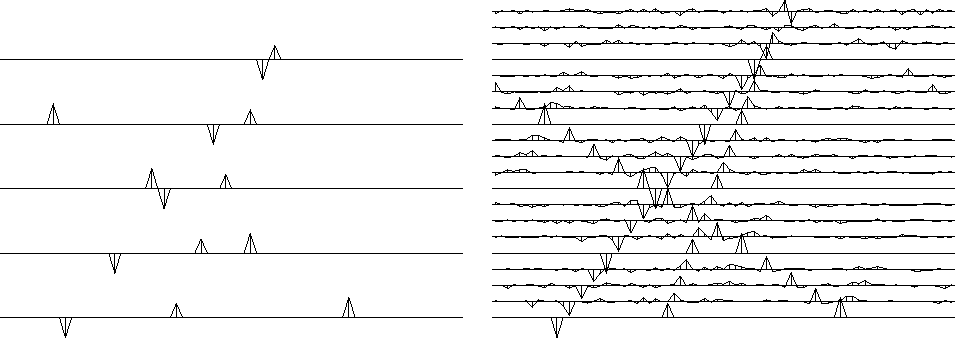
Figure 1 shows three plane waves recorded on five channels and the interpolated data.

 

lace390
Figure 1 Left is five signals, each showing three arrivals. With the data shown on the left (and no more), the signals have been interpolated. Three new traces appear between each given trace, as shown on the right.

Both the original data and the interpolated data can be described as ``beyond aliasing,'' because on the input data the signal shifts exceed the signal duration. The calculation requires only a few seconds of a two-stage least-squares method, in which the first stage estimates a PEF (inverse spectrum) of the known data, and the second uses the PEF to estimate the missing traces.

Before the method of this section can be applied to field data for migration, remember that the data must be broken into many overlapping tiles of size about like those shown here and the results from each tile pieced together.