SIGNAL-NOISE DECOMPOSITION BY DIP

Choose noise $\bold n$ to be energy that has no spatial correlation and signal $\bold s$ to be energy with spatial correlation consistent with one, two, or possibly a few plane-wave segments. (Another view of noise is that a huge number of plane waves is required to define the wavefield; in other words, with Fourier analysis you can make anything, signal or noise.) We know that a first-order differential equation can absorb (kill) a single plane wave, a second-order equation can absorb one or two plane waves, etc. In practice, we will choose the order of the wavefield and minimize power to absorb all we can, and call that the signal.

$\bold S$ is the operator that absorbs (by prediction error) the plane waves and $\bold N$ absorbs noises and $\epsilon \gt 0$ is a small scalar to be chosen. The difference between $\bold S$ and $\bold N$is the spatial order of the filters. Because we regard the noise as spatially uncorrelated, $\bold N$ has coefficients only on the time axis. Coefficients for $\bold S$are distributed over time and space. They have one space level, plus another level for each plane-wave segment slope that we deem to be locally present. In the examples here the number of slopes is taken to be two. Where a data field seems to require more than two slopes, it usually means the ``patch'' could be made smaller.

It would be nice if we could forget about the goal (12) but without it the goal (11), would simply set the signal $\bold s$equal to the data $\bold d$.Choosing the value of $\epsilon$ will determine in some way the amount of data energy partitioned into each. The last thing we will do is choose the value of $\epsilon$,and if we do not find a theory for it, we will experiment.

The operators $\bold S$ and $\bold N$can be thought of as ``leveling'' operators. The method of least-squares sees mainly big things, and spectral zeros in $\bold S$ and $\bold N$tend to cancel spectral lines and plane waves in $\bold s$ and $\bold n$.(Here we assume that power levels remain fairly level in time. Were power levels to fluctuate in time, the operators $\bold S$ and $\bold N$should be designed to level them out too.)

None of this is new or exciting in one dimension, but I find it exciting in more dimensions. In seismology, quasisinusoidal signals and noises are quite rare, whereas local plane waves are abundant. Just as a short one-dimensional filter can absorb a sinusoid of any frequency, a compact two-dimensional filter can absorb a wavefront of any dip.

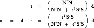
To review basic concepts, suppose we are in the one-dimensional frequency domain. Then the solution to the fitting goals (12) and (11) amounts to minimizing a quadratic form by setting to zero its derivative, say

$$0 \eq {\partial \ \over \partial \bold s'} \left( (\bold s'... ...\bold d ) + \epsilon^2 \bold s' \bold S'\bold S \bold s \right)$$ (13)

which gives the answer

$$\begin{eqnarray} \bold s &=& \left( \bold N' \bold N \over \bold N' \bold N ... ...ld N' \bold N \ + \ \epsilon^2 \bold S'\bold S \right) \ \bold d\end{eqnarray}$$ (14) (15)

To make this really concrete, consider its meaning in one dimension, where signal is white $\bold S'\bold S=1$ and noise has the frequency $\omega_0$,which is killable with the multiplier $\bold N'\bold N=(\omega-\omega_0)^2$.Now we recognize that equation (14) is a notch filter and equation (15) is a narrow-band filter.

The analytic solutions in equations (14) and (15) are valid in 2-D Fourier space or dip space too. I prefer to compute them in the time and space domain to give me tighter control on window boundaries, but the Fourier solutions give insight and offer a computational speed advantage.

Let us express the fitting goal in the form needed in computation.  

$$\left[ \begin{array} {c} \bold 0 \\ \bold 0 \end{array... ...array} {c} -\bold N \bold d \\ \bold 0 \end{array} \right]$$ (16)

Subroutine signoi2() using pef2() first computes the prediction-error filters $\bold S$ and $\bold N$.Then it loads the residual vector $\bold r$with the negative of the noise whitened data $-\bold N\bold d$.Then it enters the usual conjugate-direction iteration loop where it makes adjustments of $\Delta \bold r$ and $\Delta \bold s$.Finally, it defines noise by $\bold n = \bold d-\bold s$.

 

# Decompose data into signal and noise, d=s+n given PEF size (s1,s2) of signal.
#
subroutine signoi2( d, s, n,d1,d2,  epsilon, niter, s1,s2)
integer                     d1,d2,           niter, s1,s2, n1,n2, ls1,ln1
real d(d1*d2), s( d1*d2), n(d1*d2), epsilon
integer                                    i, iter, d12, r12, rs,rn
temporary real                 rr( d1*d2*2),   ss(s1,s2),    nn(s1,1)
temporary real     ds( d1,d2), dr( d1*d2*2), sfre(s1,s2),  nfre(s1,1)
temporary real     ps( d1,d2), pr( d1*d2*2)
                  d12= d1*d2;  r12=d1*d2;     rs=1;     rn= 1 + r12
ls1= 1+s1/2;    n1=ls1;    n2=1;   ln1=1
call setfree(ls1,1,1,sfre,s1,s2,1,i); call pef2(s,rr,d1,d2,i,ls1,1,sfre,ss,s1,s2)
call setfree(ln1,1,1,nfre,n1,n2,1,i); call pef2(n,rr,d1,d2,i,ln1,1,nfre,nn,n1,n2)

call scaleit( epsilon, s1*s2, ss)
call null( s, d12); call null( rr, 2* r12)
call         icai2(  0,0,1,1, nn,n1,n2,            d, d1,d2,  rr(rn ))
call       scaleit( -1.,                              d1*d2,  rr(rn ))
do iter= 0, niter {
        call icai2(  1,0,1,1, nn,n1,n2,            ds,d1,d2,  rr(rn ))
        call icai2(  1,1,1,1,           ss,s1,s2,  ds,d1,d2,  rr(rs ))
        call icai2(  0,0,1,1, nn,n1,n2,            ds,d1,d2,  dr(rn ))
        call icai2(  0,0,1,1,           ss,s1,s2,  ds,d1,d2,  dr(rs ))
        call cgplus( iter,   d12, s,ds,ps, _
                           2*r12, rr,dr,pr )
        }
do i=1, d12 { n(i) = d(i) - s(i) }
return; end

As with the missing-data subroutines, the potential number of iterations is large, because the dimensionality of the space of unknowns is much larger than the number of iterations we would find acceptable. Thus, sometimes changing the number of iterations niter can create a larger change than changing epsilon.

Subroutine signoi2() is set up in a bootstrapping way. It uses not only data, but also signal and noise. The first time in, I used a crude estimate of the signal and noise that is merely a copy of the raw data. Notice that these copies are used only to compute $\bold S$ and $\bold N$,the signal and noise whiteners. Because the program uses models of signal and noise to enhance the separation of signal and noise, we might consider a second invocation of the program. I tried multiple invocations to little avail. Another thing for contemplation is some automatic way of choosing $\epsilon$.