Introduction

Robust error measures such as the l¹ norm have found a number of uses in geophysics. As measures of data misfit, they show considerably less sensitivity to large measurement errors than does the mean square (l²) measure. Since geophysical inverse problems are generally ill-posed, relatively noise insensitive misfit measures can yield far more stable estimates of Earth parameters than does the mean square measure Chapman and Barrodale (1983); Claerbout and Muir (1973); Scales et al. (1988); Scales and Gersztenkorn (1988); Taylor et al. (1979). This insensitivity to large noise has a statistical interpretation: robust measures are related to long-tailed density functions in the same way that the mean square is related to the (short-tailed) Gaussian Tarantola (1987).

A simple choice of robust measure is the l¹ norm: denoting the residual (misfit) components by $r_i,\,i=1,...,N$, l¹ norm of the residual vector is $\sum_{i=1}^N\vert r_i\vert$. This function is not smooth: it is singular where any residual component vanishes. As a result, numerical minimization is difficult. Various approaches based for example on a linear programming viewpoint Barrodale and Roberts (1980) or iterative smoothing Scales et al. (1988), have been used with success but require considerable tuning. Moreover, the singularity implies that small residuals are ``taken as seriously'' as large residuals, which may not be appropriate in all circumstances.

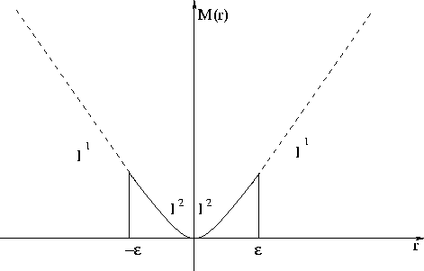
These drawbacks of the l¹ norm have led to various proposals which combine robust treatment of large residuals with Gaussian treatment of small residuals. In the work reported here, we use a hybrid l¹-l² error measure proposed by Huber Huber (1973):

$$M_{\epsilon}(r) = \left\{ \begin{array} {cc} \frac{r^2}{2\ep... ...frac{\epsilon}{2}, & \epsilon < \vert r\vert \end{array}\right.$$

We will call $\sum_{i=1}^N\,M_{\epsilon}(r_i)$ the Huber misfit function, or Huber function for short (Figure 1). Note that the Huber function is smooth near zero residual, and weights small residuals by mean square. It is reasonable to suppose that the Huber function is easier to minimize than l¹ while still robust against large residuals.

This paper describes the application of the Huber misfit function to velocity analysis. Estimation of RMS velocity (or slowness) can be posed as a linear inverse problem through the velocity transform described in the next section. Definition of the misfit via the Huber function (or any other robust error measure) results in a nonlinear optimization problem for the velocity model. This nonlinearity would seem to compare unfavorably with the least squares (l²) treatment of the same problem, which leads to a linear system (the normal equation) and so can be solved by efficient iterative methods such as conjugate gradient. We show that use of an appropriate nonlinear optimization method gives a Huber-based solution with comparable efficiency to that of conjugate gradient least squares solution. Thus the noise rejection properties of the Huber misfit function come at no appreciable premium in computational effort.

 

huber Figure 1 Error measure proposed by Huber Huber (1973). The upper part above $\epsilon$ is the l1 norm while the lower part is the l2 norm.

In the work reported here we have used a version of the Limited Memory BFGS algorithm Nocedal (1980) as implemented in the Hilbert Class Library Gockenbach et al. (1999). Other nonlinear iterative optimizers could be used; we have solved the same examples with nonlinear conjugate gradient methods Fletcher (1980) and obtained comparable results. We note that specially adapted Huber minimizers have been suggested Ekblom and Madsen (1989). One of our questions in beginning this work was whether a standard quasi-Newton method, as opposed to a special solver, would perform satisfactorily in Huber estimation.

The second section of the paper explains the velocity transform and formulates a linear inverse problem for velocity analysis. The third and fourth sections present synthetic and field data examples.