


Next: Global Analysis of Stationary
Up: Symes: Differential semblance
Previous: Noise Free Data
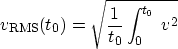
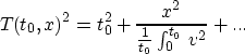
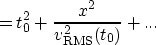
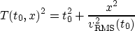
Claim: To good
approximation, for ``small'' offsets,

where the RMS velocity is
Justification [Continuum derivation of the hyperbolic
moveout
approximation]: The 2-way traveltime 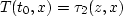 from the
surface at z=0 to depth z and back at offset x is related to the
solution of the eikonal equation
from the
surface at z=0 to depth z and back at offset x is related to the
solution of the eikonal equation  with point source at
z=x=0 by
with point source at
z=x=0 by
Thus
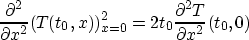
Differentiate this twice with respect to x and use the vanishing of
odd-order x derivatives at x=0 (implied by symmetry) to conclude
that the second x derivative
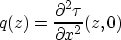
satisfies
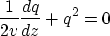
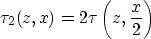
Introduce temporarily a new depth coordinate
Then in terms of  , q satisfies the Ricatti equation

The solution which is singular at  , i.e. z=0, is
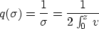
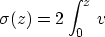
Since  , you can also write this as
Thus
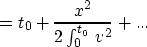
Since
the above can be rewritten
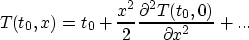
which reveals that the hyperbolic moveout approximation is just the second order
Taylor expansion of T2 in x, which should be good for ``small'' x.
This report adopts the hyperbolic moveout approximation, i.e. truncate the Taylor expansion
above and take
This amounts to assuming that all events in the data have precisely
hyperbolic moveout. Of course this assumption is not entirely consistent with
geometric optics. It has been suggested that the deviation of actual two-way
time from the hyperbolic moveout approximation may be mistaken for evidence of anisotropy
in some cases. In any case the error caused by replacing actual two way
time by its hyperbolic moveout approximation is not an asymptotic error in the
sense of the last section, so I will treat it as a component of data noise.
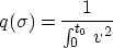
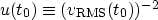
The reciprocal square RMS velocity, or RMS square slowness
is the primary expression of velocity
in the above formula. It occurs so often as to warrant its own notation:
The conditions defining the mute can be restated: since
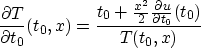
the quantity on the right hand side of this equation must be bounded
away from zero. Since v generally increases with depth, hence u
decreases, such a lower bound will only be possible for t0
exceeding a threshold for each x, which is the mute boundary
mentioned before. In the data, i.e. (t,x),
coordinates, the stretch factor condition becomes

and as before the mute  must be supported in the set specified
by this condition.
must be supported in the set specified
by this condition.
The upper and lower velocity envelopes implied by membership of
the velocity in  imply
corresponding envelope mean square slownesses
(
imply
corresponding envelope mean square slownesses
( corresponding to
  and vis-versa) so that
 .
.
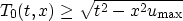
It is usually reasonable to assume the lower velocity bound to be
constant (independent of t0) - for example, equal to sound velocity
in water, or close to it. Then  is also constant, so
you can explicitly estimate a lower bound for T0:
is also constant, so
you can explicitly estimate a lower bound for T0:

so
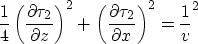
The velocity bounds also imply a bound on the derivative of u:

The bounds on v, the known value of v at the surface,
and the maximum two way time imply bounds on the slope
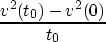
whence a bound  on the derivative of u follows
immediately.
on the derivative of u follows
immediately.
Since both the lower bound on T0 and the uppoer bound on
the derivative of u are uniform over , a -uniform
bound on the stretch factor follows:
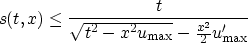
From this you can derive a -uniform mute boundary. Therefore
assume henceforth that is a -uniform mute.
Next: Global Analysis of Stationary
Up: Symes: Differential semblance
Previous: Noise Free Data
Stanford Exploration Project
4/20/1999