Results

According to Koefoed's conclusion mentioned by Shuey (1985), when the underlying medium has a greater longitudinal velocity and a greater Poisson's ratio, the reflection coefficient tends to increase with increasing angles of incidence. We could expect this AVO behavior at the flat reflector, assuming the hypothesis Ecker (1998) that this reflector marks the transition from gas-saturated to brine-saturated sediments, and because gas-saturated sediments exhibit abnormally low Poisson ratios Ostrander (1984).

However, in Figure 9 we can see that the general tendency has the opposite behavior-decreasing amplitude values with increasing offset ray parameter-even though in the near offset the reflection coefficient tends to increase with increasing offset ray parameter, as expected. There are several possible explanations for this discrepancy. Perhaps the original hypothesis-that the flat reflector marks the transition from gas-saturated to brine-saturated sediments-doesn't hold. On the other hand, the discrepancy may be the result of procedural problems associated, for example, with the fact that the attributes we considered are not strictly AVO attributes.

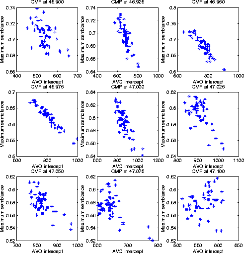
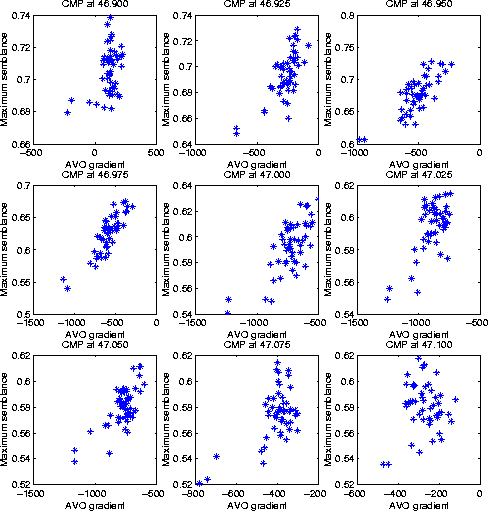
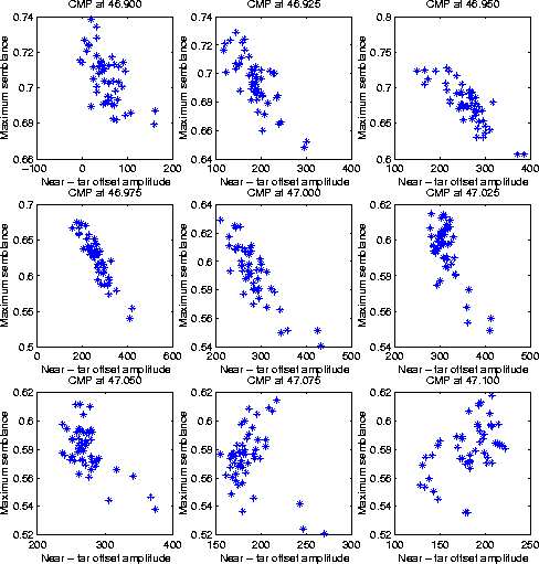
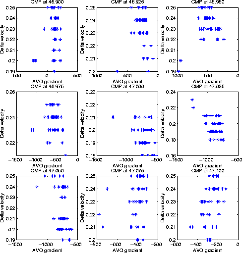
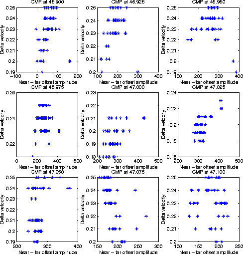
From the calculated coherence measures and attribute values at some CMPs around distance 47 km, we generated the crossplot of attribute versus coherence shown in Figures 10 through 15. In general, it is difficult to establish definitive tendencies of attributes and velocity coherence. However, for the case of maximum semblance coherence measures, as is shown in Figures 10, 11, and 12, attribute values are more dispersed for lower coherence values, and more localized for higher coherence values. 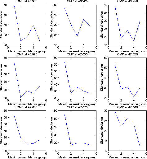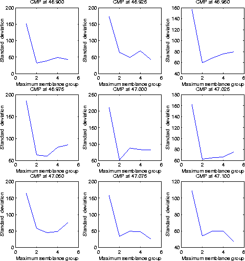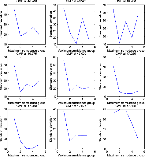We sorted the coherence values and generated five groups of data samples, then calculated the variance and standard deviation for each group. For the case of the maximum semblance, the results suggest that attribute values tend to have higher variance and higher standard deviation as coherence values decrease. Figures 16, 17, and 18 show the standard deviation results corresponding to the maximum semblance plots in Figures 10, 11, and 12.

 

int-max
Figure 10 Intercept versus maximum semblance for CMPs from 46.9 to 47.1 km

 

grad-max
Figure 11 Gradient versus maximum semblance for CMPs from 46.9 to 47.1 km

 

stack-max
Figure 12 Near - far offset amplitude versus maximum semblance for CMPs from 46.9 to 47.1 km

 

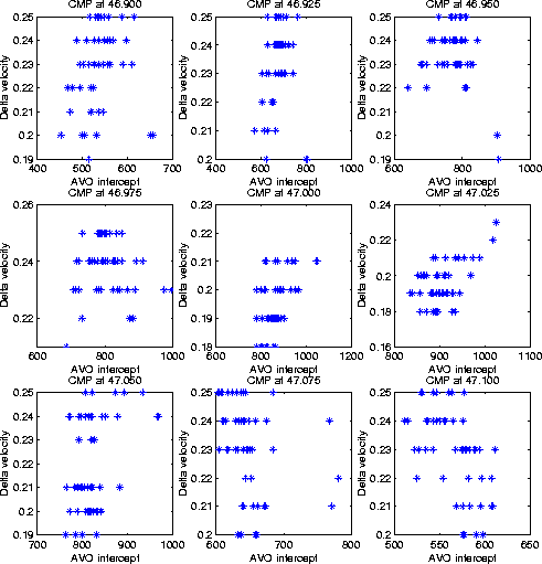
int-delta
Figure 13 Intercept versus delta velocity for CMPs from 46.9 to 47.1 km

 

grad-delta
Figure 14 Gradient versus delta velocity for CMPs from 46.9 to 47.1 km

 

stack-delta
Figure 15 Near - far offset amplitude versus delta velocity for CMPs from 46.9 to 47.1 km

 

std
Figure 16 Maximum semblance group versus standard deviation corresponding to plots in Figure 10

 

std2
Figure 17 Maximum semblance group versus standard deviation corresponding to plots in Figure 11

 

std3
Figure 18 Maximum semblance group versus standard deviation corresponding to plots in Figure 12