


Next: Non-stationary convolution and combination
Up: Theory
Previous: Theory
The convolution of a vector,
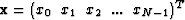 ,
with a causal filter,
,
with a causal filter,
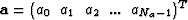 ,whose first element, a0=1, and whose length, Na<N,
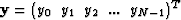
onto an output vector,
,whose first element, a0=1, and whose length, Na<N,
onto an output vector,
 ,
can be defined by the set of equations:
,
can be defined by the set of equations:
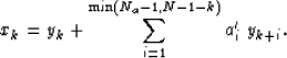
| 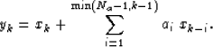 |
(1) |
This can be rewritten in linear operator notation, as
 , where
  is a lower-triangular
Toeplitz matrix representing convolution with the filter,
is a lower-triangular
Toeplitz matrix representing convolution with the filter,  .
.
The adjoint operator,  , which describes time-reversed
filtering with filter , can similarly be expressed by
considering the rows of the matrix-vector equation,
, which describes time-reversed
filtering with filter , can similarly be expressed by
considering the rows of the matrix-vector equation,
 , as follows,
|  |
(2) |
The helicon Fortran90 module Claerbout (1998a) exactly implements the
linear operator (and adjoint) pair described by
equations (1) and (2).
Equation (1) explicitly prescribes internal boundary
conditions near k=0; however, since is causal, no
particular care is needed near k=N-1. On the other hand,
equation (2) explicitly imposes internal boundary
conditions near k=N-1, and no care is needed near k=0.
It is possible to rewrite equations (1)
and (2) in a more symmetric form; however, as written,
the equations lead naturally to recursive inverses for operators,
and .
Rearranging equation (1), we obtain
| 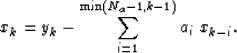 |
(3) |
This provides a recursive algorithm, starting from x0=y0 for
solving the system of equations, .Equation (3) describes the exact, analytic inverse of
causal filtering with equation (1).
In principle, given a filter, , and a filtered trace,
 , the above equation can recover the unfiltered trace,
 exactly; although in practice, with numerical errors, the
division may become unstable if is not minimum phase.
Similarly, if we inverse filter a trace with
equation (3), we can recover the original by causal
filtering with equation (1) subject to the stability of
the inverse filtering process.
exactly; although in practice, with numerical errors, the
division may become unstable if is not minimum phase.
Similarly, if we inverse filter a trace with
equation (3), we can recover the original by causal
filtering with equation (1) subject to the stability of
the inverse filtering process.
Equation (3) appears very similar to polynomial
division. However, the output of polynomial division is an infinite
series, while equation (3) is defined only in the
range,  . As such, equation (3)
describes polynomial division followed by truncation.
. As such, equation (3)
describes polynomial division followed by truncation.
Equation (2) can also be rewritten as
| 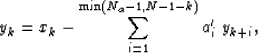 |
(4) |
which provides an exact recursive inverse to adjoint operator,
, that can be computed starting from yN-1=xN-1, and
decrementing k.
Next: Non-stationary convolution and combination
Up: Theory
Previous: Theory
Stanford Exploration Project
10/25/1999