


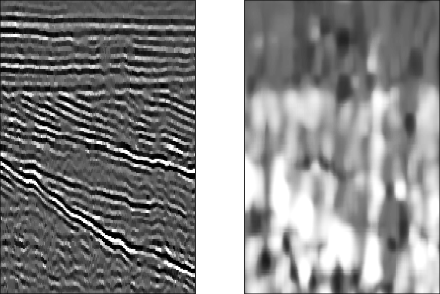
Figure 7 shows the real 2-D seismic image and its associated local dip estimate. The image processed here is a 200x200 subwindow from a migrated 2-D section originally acquired by Mobil over a Gulf of Mexico prospect. The upper portion of the windowed data is characterized by an unconformity. Figure 8 shows the facies template used to test the algorithm and the corresponding local dip estimate. The 50x50 template was created artificially and is designed to resemble the unconformity in the data.
 |


|
seis-trnshow
Figure 8 Left: Facies templates, corresponding to the unconformities in the upper part of the data (Figure 7). Right: Estimated local dip. | 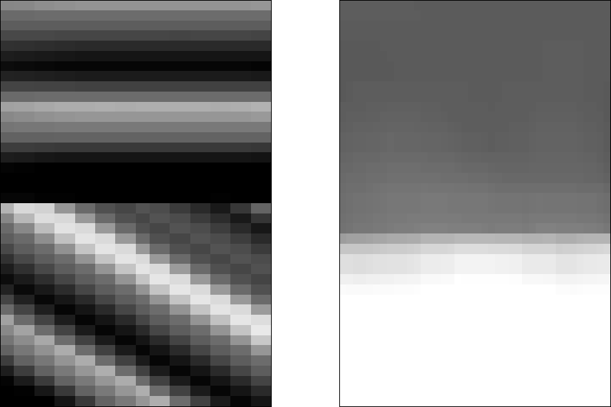 |
The quality of the dip estimates is critical to the success of the algorithm, but unfortunately these estimates are more prone to error with real data than they are for synthetic data (Compare Figures 3 and 7). In order to maximize the spatial coherency of the input data, and hence the robustness of the dip estimate, some smoothing of the data may be required prior to processing. In this case, the estimated dip field was smoothed using a local weighted mean filter, where the weights are the so-called ``normalized correlation'' measure of Claerbout (1992) - roughly speaking, a measure of the data's local ``plane-waveness''.
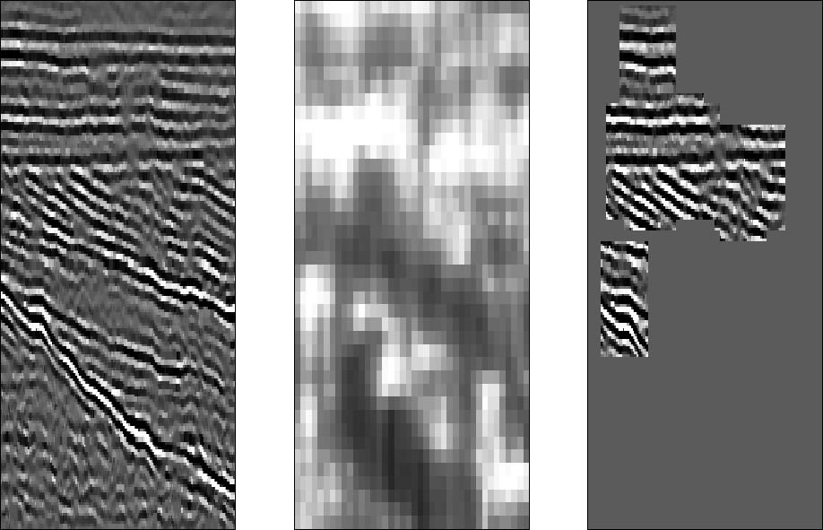
Figure 9 shows the output of the pattern recognition program. The results are good, having effectively done the same job as a human interpreter, even with a less-than-perfect dip estimate (Figure 8).
 |