The Iteratively Reweighted Least Square method

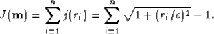
The IRLS implementation of the hybrid l²-l¹ norm differs greatly from the Huber solver. In this section, I follow quite closely what Nichols (1994) and Darche (1989) suggested in previous reports. The main idea is that instead of minimizing the simple l² norm, we can choose to minimize a weighted residual. The objective function becomes

$$f(\bold{m})= \Vert\bold{WHm}-\bold{Wd}_{obs}\Vert _2.$$ (4)

A difference between the Huber solver and IRLS clearly arises here since we still solve a least-square problem with IRLS and not with the Huber solver. The IRLS method weights residuals within a linear l² framework and Huber uses either l² or l¹ following the residual with a nonlinear update. A particular choice for $\bold{W}$ will lead to the minimization of the l²-l¹ norm, however. In this paper, I choose

$$\begin{eqnarray} w_{ii}=\frac{1}{[1+(r_{ii}/\epsilon)^2]^{1/4}},\end{eqnarray}$$ (5)

with $r_i=\bold{Hm}_i-\bold{d}_i$ and $\epsilon$ a damping parameter. With this particular choice of W, minimizing f is equivalent to minimizing Bube and Langan (1997)

$$J(\bold{m})=\sum_{i=1}^{n}j(r_i)=\sum_{i=1}^{n}\sqrt{1+(r_i/\epsilon)^2}-1.$$ (6)

For any given residual r_i, we notice that

$$j(r) \approx \left\{ \begin{array} {cc} \frac{1}{2}(r/\epsi... .../\epsilon & \mbox{for \vert r\vert large.} \end{array} \right.$$

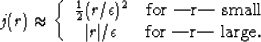
Hence, we obtain a l¹ treatment of large residuals and a l² treatment of small residuals. Darche (1989) gives a practical value for $\epsilon$ that can be also used for the Huber threshold:

$$\epsilon = \frac{max\vert\bold{d}\vert}{100}.$$

Two different IRLS algorithms are suggested in the literature Scales and Gersztenkorn (1988). The first method consists of solving successive l² problems with a constant weight and taking the last solution obtained to recompute the weight for the next l² problem. The second method consists of recomputing the weights at each iteration (in fact, we need only a few iterations of the conjugate gradient scheme before calculating the new weight), solving small piecewise linear problems. The IRLS algorithms converge if each minimization reaches a minimum for a constant weight Bube and Langan (1997). This is the case for the first method described above, but it is also true for the second method since each starting point of the next iteration is the ending point of the previous solving piecewise linear problems. For practical reasons, we utilize the second method. Indeed, for most geophysical problems, the complete solution of the l² problem with a constant weight would lead to prohibitive costs. The general process in the program is as follows:

1.

compute the current residual $\bold{r}=\bold{Hm}-\bold{d}$

2.

compute the weighting operator $\bold{W}$ using $\bold{r}$

3.

solve the weighted least-squares problem (equation 4) using a Conjugate Gradient algorithm

4.

go to first step

We do not detail the Conjugate Gradient step here. For more details, the reader may refer to Paige and Saunders (1982). In our implementation, we control the restarting schedule of the iterative scheme with one parameter that governs the periodic computing of the weight. The Conjugate Gradient is reset for each new weighting function, meaning that the first iteration of each new least-squares problem (for each new weight) is a steepest descent step. In addition, the last solution $\bold{m}$ of the previous least-squares problem is used to compute the new residual and the new weighting matrix (steps 1 and 2 in the IRLS algorithm). In the following examples, except when indicated, we recompute the weight every five iterations. In the following sections, I call ``IRLS'' the IRLS algorithm described above with the weighting function in equation (5).