Minimizing the Huber function

In the work reported here, I use a hybrid l¹-l² error measure proposed by Huber Huber (1973):

$$M_{\epsilon}(r) = \left\{ \begin{array} {cc} \frac{r^2}{2\ep... ...frac{\epsilon}{2}, & \epsilon < \vert r\vert \end{array}\right.$$

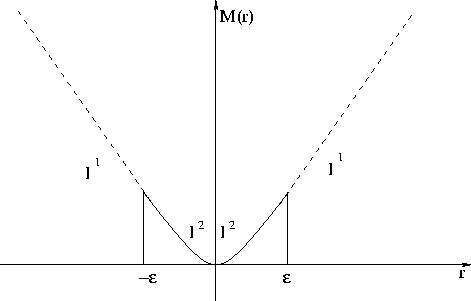
I will call $\sum_{i=1}^N\,M_{\epsilon}(r_i)$ the Huber misfit function $H_\epsilon$,or Huber function for short (Figure 1). Note that the Huber function is smooth near zero residual, and weights small residuals by the mean square. It is reasonable to suppose that the Huber function, while maintaining robustness against large residuals, is easier to minimize than l¹. The parameter $\epsilon$, which controls the limit between l¹ and l², is called the Huber threshold.

 

huber Figure 1 Error measure proposed by Huber Huber (1973). The upper part above $\epsilon$ is the l1 norm, while the lower part is the l2 norm.

The problem is this: given some observed data $\bold{d}_{\bf obs}$, we want to find the best model $\bold{m}$ that explains the data via the operator $\bold{H}$. This may be posed in terms of an inverse problem leading to the minimization of the function

$$f(\bold{m})= E(\bold{Hm}-\bold{d}_{\bf obs}),$$ (1)

where E is an error measure function. As discussed above, I will use the Huber function and try to minimize

$$f(\bold{m}) = H_{\epsilon}(\bold{Hm}-\bold{d}_{\bf obs}).$$ (2)

We seek to find the stationary point $\bold{m}^{\ast}$ of the function f. This solution point satisfies $\bold{f}'(\bold{m}^{\ast})=\bold{0}$. This is a nonlinear system of equations, and from Taylor expansion we have

$$\bold{f}'(\bold{m+\delta m})\simeq \bold{f}'(\bold{m})+\bold{f}''(\bold{m})\delta \bold{m}$$

if $\Vert\delta \bold{m}\Vert$ is sufficiently small. The Newton's method consists in finding $\delta \bold{m}$ such that

$$\bold{H} \delta \bold{m} = -\bold{f}'(\bold{m}) \mbox{ with } \bold{H}=\bold{f}''(\bold{m}),$$

and computing the next iterate by

$$\bold{m}_{n+1}=\bold{m}_{n}+\alpha_n\delta \bold{m}_n$$ (3)

where $\alpha_n$ is a steplength given by a Line Search algorithm. The general process of the program is then

1.

compute the gradient $\bold{f}'(\bold{m})$

2.

compute $\delta \bold{m}_n = - \bold{H}^{-1}\bold{f}'(\bold{m})$

3.

compute $\alpha_n$ using a line search

4.

update the solution $\bold{m}_{n+1}=\bold{m}_{n}+\alpha_n\delta \bold{m}_n$

5.

update the Hessian $\bold{H}$

6.

go to 1.

Because the Huber function is not twice continuously differentiable, the Hessian is not computed directly but approximated using a limited Memory BFGS update Guitton (2000), as proposed by Nocedal (1980) and Liu and Nocedal (1989). I have implemented for the line search a More and Thuente More and Thuente (1994) algorithm, which ensures sufficient decrease for the function f and obeys curvature conditions (the so-called Wolfe conditions, Kelley (1999)), thus guaranteeing that a quasi-Newton update is possible. The steplength $\alpha_n = 1$ is always tried first, saving significant computation. These choices lead to good performances for both convergence rate and computation cost. I call ``Huber solver'' the algorithm detailed above when used with the Huber norm.