Tests on synthetic data: spiky events

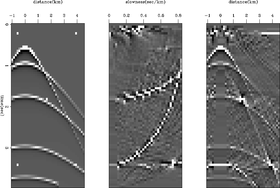
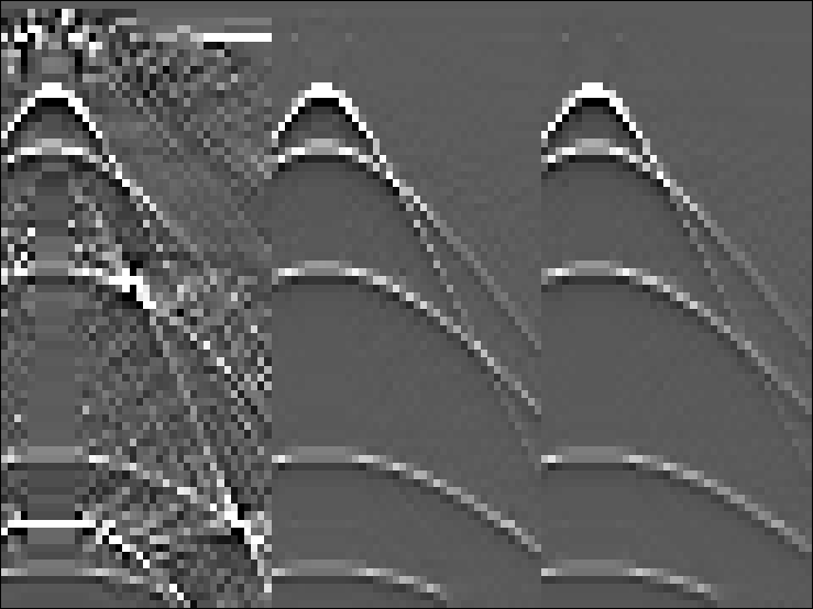
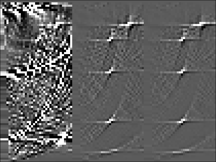
Figure 2 shows the input data for the first synthetic example plus the l² inversion result; it demonstrates the sensitivity of least-squares to outliers: some ellipses appear in the model space and the data space is infested with noise. Figures 3 and 4 show a comparison between IRLS and the Huber solver (same clip applied on the data). The damping parameter for IRLS and the Huber threshold were chosen as suggested above ($\epsilon=max\vert\bold{d}\vert/100$). Both results are very comparable since we get rid of the spikes in the data space (Figure 3). In addition, the five expected velocity events, associated with the five input hyperbolas, are clearly identifiable in the model space (Figure 4). Both results are very conclusive since the spikes have been correctly ``l¹ handled''.

 

gr-spiky-L2-HUBER
Figure 2 From left to right: 1) Input data. 2) velocity domain, l² inversion result. 3) remodeled data from the l² result

 

comp-data-spiky-0.04
Figure 3 From left to right: 1) Remodeled data with l². 2) Remodeled data with the Huber solver. 3) Remodeled data using IRLS

 

comp-mod-spiky-0.04
Figure 4 From left to right: 1) l² velocity space. 2) Huber velocity space. 3) IRLS velocity space