


Next: Lemma
Up: Guitton: Huber solver
Previous: Proof
We will assume that f and  satisfy the following assumptions:
- 1.
- f is twice continuously differentiable
- 2.

- 3.
 is symmetric positive definite
The Newton methods update the current iteration  by the formula
|  |
(1) |
where  is given by a line search that ensures sufficient decrease.
Quasi-Newton methods update an approximation of the Hessian
is given by a line search that ensures sufficient decrease.
Quasi-Newton methods update an approximation of the Hessian  as the iterations
progress. A possible update is the BFGS method Broyden (1969); Fletcher (1970); Goldfarb (1970); Shanno (1970), which
overcomes some limitations of the earlier Broyden's method Broyden (1965).
In particular, the Broyden's update does not keep the spd structure of the Hessian.
This structure not only ensures the existence of a local minimizer but also allows the convergence
of the updated solution
as the iterations
progress. A possible update is the BFGS method Broyden (1969); Fletcher (1970); Goldfarb (1970); Shanno (1970), which
overcomes some limitations of the earlier Broyden's method Broyden (1965).
In particular, the Broyden's update does not keep the spd structure of the Hessian.
This structure not only ensures the existence of a local minimizer but also allows the convergence
of the updated solution  to the minimum Kelley (1999).
The BFGS update is a rank-two update given by
to the minimum Kelley (1999).
The BFGS update is a rank-two update given by
| 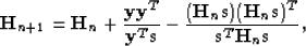 |
(2) |
with  and
and 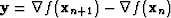 .In practice, it is very useful to express the previous equation in terms of the inverse matrices. We then have
| 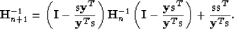 |
(3) |
Next: Lemma
Up: Guitton: Huber solver
Previous: Proof
Stanford Exploration Project
4/27/2000