L-BFGS update

For the sake of completeness, I give the updating formulas of the Hessian as presented by Nocedal (1980). We define first

$$\bold{\rho}_i = 1/\bold{y}_i^T\bold{s}_i \mbox{ and } \bold{v}_i=(I-\bold{\rho}_i\bold{y}_i\bold{s}_i^T).$$

In addition, we pose $\bold{H}^{-1}=\bold{B}$.As described above, when k, the number of iterations, obeys $k+1 \leq m$, where m is the storage limit, we have the usual BFGS update

	(4)

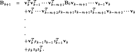
For k+1 > m we have the special limited-memory update

$$\begin{eqnarray} \bold{B}_{k+1}&=&\bold{v}_k^T\bold{v}_{k-1}^T\cdots\bold{v}_{k-... ...bold{v}_k \nonumber\\ & &+\rho_k\bold{s}_k\bold{s}_k^T. \nonumber\end{eqnarray}$$ (5)

It is easy to show that the special updated Hessian is also spd. The L-BFGS algorithm is then

Algorithm1

1.

Choose $\bold{x}_0$, m, $0<\mu<1$, $\mu<\nu<1$ and a symmetric positive definite $\bold{B}_0$. Set k=0

2.

Compute

$$\begin{eqnarray} \bold{d}_k&=&-\bold{B}_k\nabla f(\bold{x}_k)\\ \bold{x}_{k+1}&=&\bold{x}_k+\lambda_k\bold{d}_k, \end{eqnarray}$$ (6) (7)

where $\lambda_k$ verifies the Wolfe conditions More and Thuente (1994):

$$\begin{eqnarray} f(\bold{x}_k+\lambda_k\bold{d}_k) &\leq& f(\bold{x}_k) + \mu \l... ...d{d}_k\vert&\geq& \nu\vert\nabla f(\bold{x}_k)^T\bold{d}_k\vert. \end{eqnarray}$$ (8) (9)

We always try steplength $\lambda_k=1$ first.

3.

Let $\hat{m}$=min$\{k$,$m-1\}$. Check if $\bold{y}_k^T\bold{s}_k\gt$.

• If no: $\bold{B}_{k+1}=\bold{I}$ (steepest descent step) and delete the pairs $\{\bold{y}_i,\bold{s}_i\}_{j=k-\hat{m}}^k$.
• If yes: Update $\bold{B}_0$ $\hat{m}+1$ times using the pairs $\{\bold{y}_i,\bold{s}_i\}_{j=k-\hat{m}}^k$, i.e., let

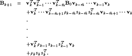
  $$\begin{eqnarray} \bold{B}_{k+1}&=&\bold{v}_k^T\bold{v}_{k-1}^T\cdots\bold{v}_{k-... ...ld{v}_k \nonumber\\ & &+\rho_k\bold{s}_k\bold{s}_k^T. \nonumber \end{eqnarray}$$ (10)

4.

Set k:=k+1 and go to 2.

The update $\bold{B}_{k+1}$ is not formed explicitly; instead, we compute $\bold{d}_k=-\bold{B}_k\nabla f(\bold{x}_k)$with an iterative formula Nocedal (1980). Liu and Nocedal (1989) propose that we scale the initial symmetric positive definite $\bold{B}_0$ at each iteration:

$$\bold{B}_k^0=\frac{\bold{y}_k^T\bold{s}_k}{\parallel\bold{y}_k\parallel^2}\bold{B}_0.$$ (11)

This scaling greatly improves the performances of the method. Liu and Nocedal (1989) show that the storage limit for large-scale problems has little effect on the method's performances. A common choice for m is m=5 (this is the default in my implementation as well). Conditions (8) and (9) are satisfied if we use an appropriate line search algorithm. I programmed a MoreThuente line search algorithm More and Thuente (1994), which ensures sufficient decrease of the objective function (equation 8) and obeys the curvature condition given in equation (9). We do not describe this program here. In practice, the initial guess $\bold{B}_0$ for the Hessian can be the identity matrix $\bold{I}$; then it might be scaled as proposed above. Liu and Nocedal (1989) prove that the L-BFGS algorithm converges to the local minimizer $\bold{x}^*$ and that the family of solutions $\{\bold{x}_k\}$ converges R-linearly (remember that the usual BFGS gives q-superlinear convergence, which is better).