Review

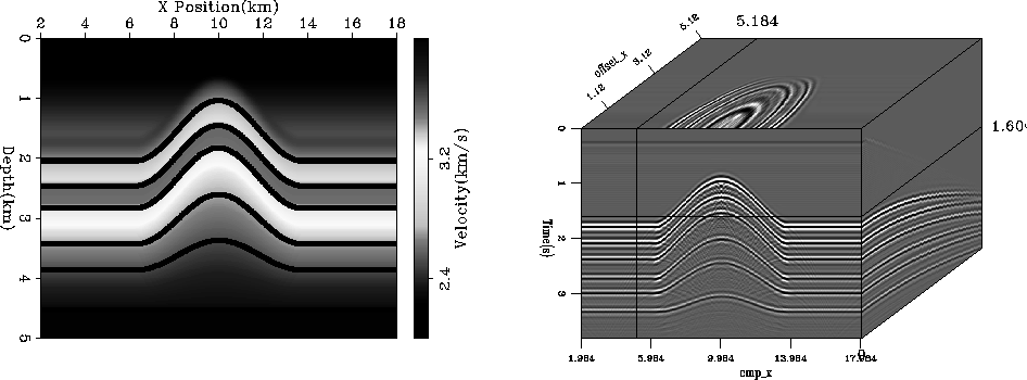
The next step is to see how well our non-stationary filter regularizes a tomography problem. I constructed a synthetic anticline model (Figure 11) with six reflectors,one above the anticline, four within the anticline, and one flat reflector representing basement rock. For added difficulty, there is a low velocity layer between the second and third reflector. 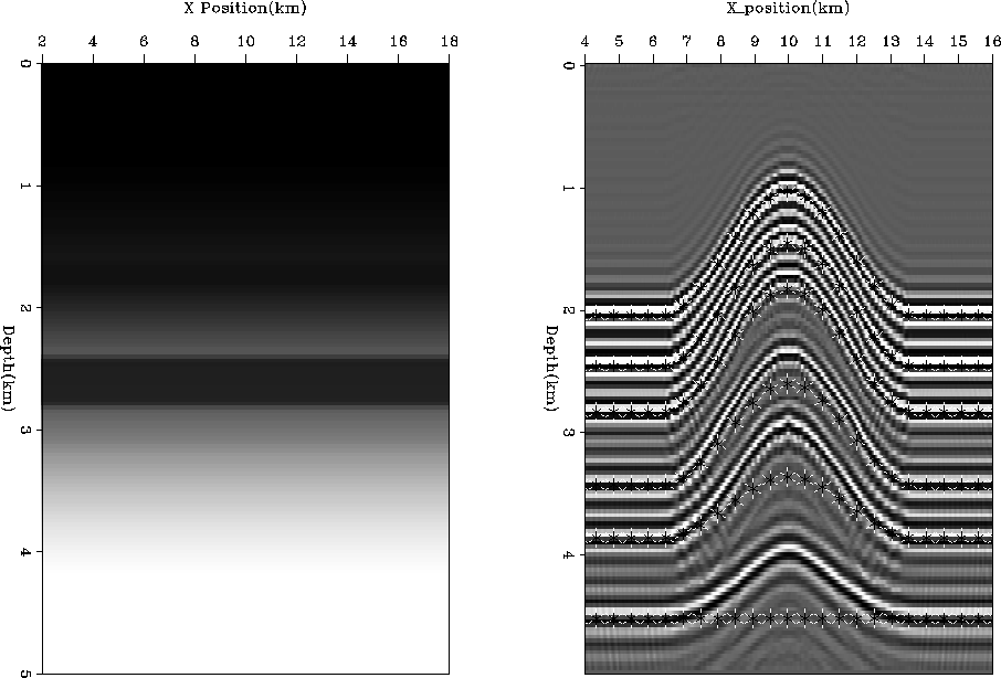The model was used to do acoustic wave modeling, with the resulting dataset having 32 meter CMP spacing and 80 offsets spaced 64 meters apart.If we use as our initial estimation of the slowness, an s(z) function from outside the anticline, the reflectors are pulled up due to using too low a velocity within the anticline (Figure 12).

 

synth-model
Figure 11 Left panel is the synthetic velocity model with six reflectors spanning the anticline. The right panel shows the data generated from this model.

 

mig0
Figure 12 Left panel is our initial guess at the velocity function, the right panel shows the zero offset ray parameter reflector position using this migration velocity. The correct reflector positions are shown as `*'. Note that reflectors are significantly mispositioned.

Following the methodology of Clapp and Biondi (1999) we will begin by considering a regularized tomography problem. We will linearize around an initial slowness estimate and find a linear operator in the vertical traveltime domain $\bf T_{}$ between our change in slowness $\bf \Delta s$and our change in traveltimes $\bf \Delta t$.We will write a set of fitting goals,

$$\begin{eqnarray} \bf \Delta t&\approx&\bf T_{} \bf \Delta s\nonumber \\ \bf 0&\approx&\epsilon \bf A\bf \Delta s,\end{eqnarray}$$ (5)

where ($\bf A$) is our steering filter operator.

However, these fitting goals don't accurately describe what we really want. Our steering filters are based on our desired slowness rather than change of slowness. With this fact in mind, we can rewrite our second fitting goal as:

$$\begin{eqnarray} \bf 0&\approx&\bf A\left( {\bf s_0} + \bf \Delta s\right) \\ -\epsilon \bf A{\bf s_0} &\approx&\epsilon \bf A\bf \Delta s.\end{eqnarray}$$ (6) (7)

Our second fitting goal cannot be strictly defined as regularization but we can do a preconditioning substitution:

$$\begin{eqnarray} \bf \Delta t&\approx&\bf T_{} \bf A^{-1}\bf p\nonumber \\ - \epsilon \bf A{\bf s_0} &\approx&\epsilon \bf I\bf p .\end{eqnarray}$$ (8)