


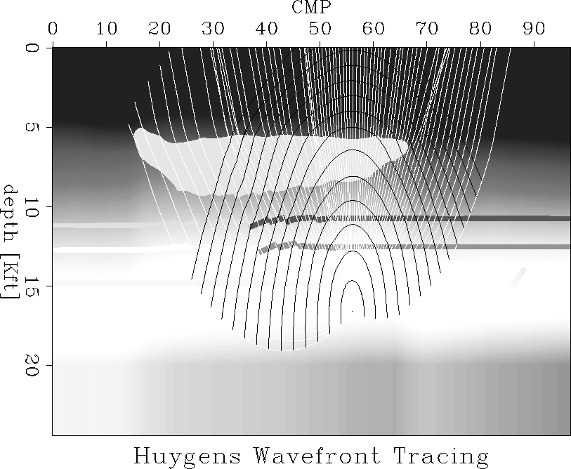
The section produced from the input CMPs and the P-wave velocity function is seen in Figure 6. This is an obvious improvement over the stacked section in Figure 5. The salt boundary has been imaged very well, including the faults at the base of the salt. Under the salt, the fault blocks to the right are imaged very well, with the two layers seen in the impedance plots very apparent in the image. However, as expected, the blocks and layers to the left are not very well imaged, because the impedance contrasts are such that not much energy is reflected.
We can also see that the part of the synclinal structure under the salt is not visible. The dips and positions of the right flank seem good, but under the salt, the image is lost. This is likely due to a problem with the raypaths being distorted as the wavefield is going through the salt. This causes less energy to get to the receivers, and thus that part of the image does not show up Muerdter et al. (1996). The same scattering effects are seen in the lens, which has a shadow zone under the salt boundary where the wavefield energy does not reach the receivers. Another feature is the trace of the salt bottom which appears just a little bit down from the bottom of the salt. This is actually the S-wave energy from the travel of converted waves in the salt which stacks at that velocity. With the exception of these shadow zone problems, and some of the S-wave energy, the image is very good when compared to the actual model.
 |


