Problem formulation

If $\bold{D}$ is a regularization operator, and $\bold{m}$ is the estimated model, then Claerbout's interpolation method amounts to minimizing the power of $\bold{D m}$ ($\bold{m}^T \bold{D}^T \bold{D m}$) under the constraint  

$$\bold{K m = m_k}\;,$$ (1)

where $\bold{m_k}$ stands for the known data values, and $\bold{K}$ is a diagonal matrix with 1s at the known data locations and zeros elsewhere. It is easy to implement a constraint of the form (1) in an iterative conjugate-gradient scheme by simply disallowing the iterative process to update model parameters at the known data locations Claerbout (1999).

The operator $\bold{D}$ can be considered as a differential equation that we assume the model to satisfy. If $\bold{D}$ is able to remove all correlated components from the model and produce white Gaussian noise in the output, then $\bold{D}^T \bold{D}$ is essentially equivalent to the inverse covariance matrix of the model, which appears in the statistical formulation of least-squares estimation Tarantola (1987).

In this paper, I propose to use the offset continuation equation Fomel (1995a) for the operator $\bold{D}$. Under certain assumptions, this equation is indeed the one that prestack seismic reflection data can be presumed to satisfy. The equation has the following form:  

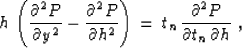$$h \, \left( {\partial^2 P \over \partial y^2} - {\partial^2 ... ...\, t_n \, {\partial^2 P \over {\partial t_n \, \partial h}} \;,$$ (2)

where P(t_n,h,x) is the prestack seismic data after the normal moveout correction (NMO), t_n stands for the time coordinate after NMO, h is the half-offset, and y is the midpoint. Offset continuation has the following properties:

• Equation (2) describes an artificial process of prestack data transformation in the offset direction. It belongs to the class of linear hyperbolic equations. Therefore, the described process is a wave-type process. Half-offset h serves as a continuation variable (analogous to time in the wave equation).
• Under a constant-velocity assumption, equation (2) provides correct reflection traveltimes and amplitudes at the continued sections. The amplitudes are correct in the sense that the geometrical spreading effects are properly transformed independently from the shape of the reflector. This fact has been confirmed both by the ray method approach Fomel (1995a) and by the Kirchhoff modeling approach Fomel et al. (1996); Fomel and Bleistein (1996).
• Dip moveout (DMO) Hale (1995) can be regarded as a particular case of offset continuation to zero offset Deregowski and Rocca (1981). As shown in my earlier paper Fomel (1995b), different known forms of DMO operators can be obtained as solutions of a special initial-value problem on equation (2).
• To describe offset continuation for 3-D data, we need a pair of equations such as (2), acting in two orthogonal projections. This fact follows from the analysis of the azimuth moveout operator Biondi et al. (1998); Fomel and Biondi (1995).
• A particularly efficient implementation of offset continuation results from a log-stretch transform of the time coordinate Bolondi et al. (1982), followed by a Fourier transform of the stretched time axis. After these transforms, equation (2) takes the form  

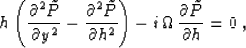  $$h \, \left( {\partial^2 \tilde{P} \over \partial y^2} - {\... ... i\,\Omega \, {\partial \tilde{P} \over {\partial h}} = 0 \;,$$ (3)

  where $\Omega$ is the corresponding frequency, and $\tilde{P} (\Omega,h,x)$ is the transformed data Fomel (1995b). As in other F-X methods, equation (3) can be applied independently and in parallel on different frequency slices.

I propose to adopt a finite-difference form of the differential operator (3) for the regularization operator $\bold{D}$. A simple analysis of equation (3) shows that at small frequencies, the operator is dominated by the first term. The form ${\partial^2 P \over \partial y^2} - {\partial^2 P \over \partial h^2}$ is equivalent to the second mixed derivative in the source and receiver coordinates. Therefore, at low frequencies, the offset waves propagate in the source and receiver directions. At high frequencies, the second term in (3) becomes dominating, and the entire method becomes equivalent to the trivial linear interpolation in offset. The interpolation pattern is more complicated at intermediate frequencies.