Missing data example

The missing data problem is probably the simplest to understand and interpret. Following the methodology of Claerbout (1999) we solve the problem in its preconditioned form using

$$\begin{eqnarray} \bf d&\approx& \bf J \bf A^{-1}\bf p\ \nonumber \bf 0&\approx& \bf I\bf p ,\end{eqnarray}$$ (3)

where:

$\bf d$

is a binned version of our known points

$\bf J$

is the known data selector

$\bf A^{-1}$

is the preconditioning operator (in this case equation (2))

p

is our preconditioned variable.

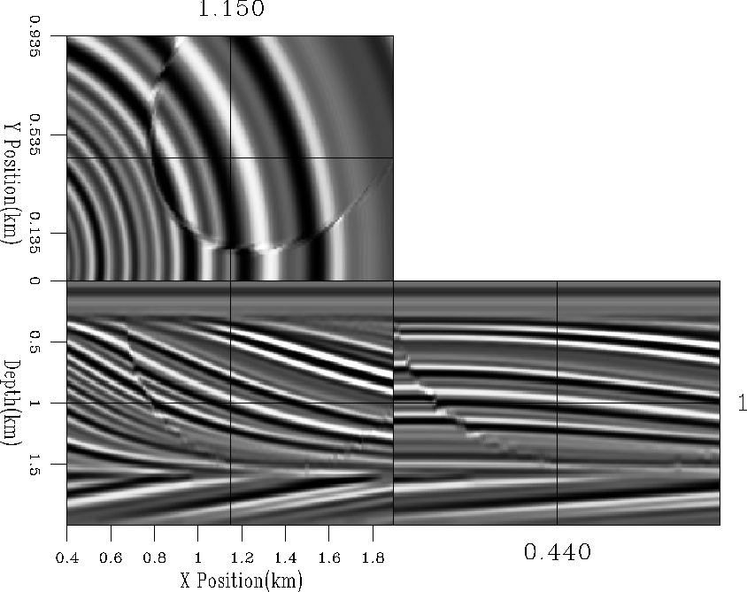
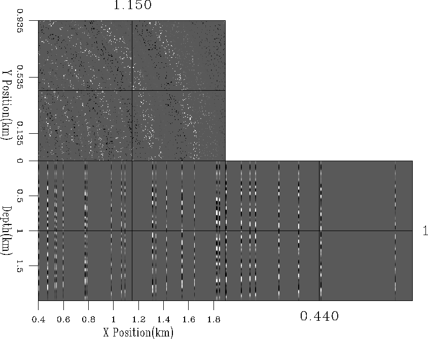
To test the interpolation I used the `qdome' dataset (Figure 4). I began by zeroing 95% of the original data (Figure 5) in vertical sections (somewhat simulating well logs). To obtain the p_xz and p_yz dip field I used the same methodology as Fomel (1999) estimating the dip field from the known data using a non-linear estimation scheme.

 

mod-orig
Figure 4 3-D qdome model from Claerbout (1999).

 

mod-in
Figure 5 Decimated qdome model. 95% of the original traces (Figure 4) have been thrown away.

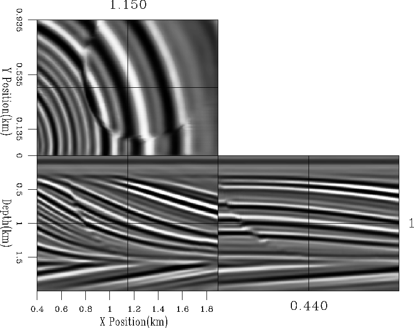
Using the calculated dip field I then constructed $\bf A_x$ and $\bf A_y$ and iterated 50 times using fitting goals (4). Figure 6 shows the resulting interpolation. In general the 3-D steering filters did an excellent job recovering the original data. There is some lower frequency behavior around the fault boundaries but the fault position is still quite obvious.

 

mod-out
Figure 6 Interpolated qdome model starting from the data in Figure 5. Note how it is a little lower frequency than Figure 4 but otherwise a near perfect interpolation result.