Super Dix

In general the operator $\bf L$ in fitting goals (7) is much more complex than the simple masking operator used in the missing data problem. One of the most attractive potential uses for a range of equiprobable models is in velocity estimation. As a result I decided to next test the methodology on one of the simplest velocity estimation operators, the Dix equation Dix (1955).

Following the methodology of Clapp et al. (1998), I start from a CMP gather q(t,i) moveout corrected with velocity v. A good starting guess for our RMS velocity function is the maximum ``instantaneous stack energy'',

$${\rm stack}(t,v) = \sum_{i=0}^n {\rm NMO_v}(q(t,i)) .$$ (9)

Not all times have reflections so we don't weight each $v_{\rm rms}(t)$ equivalently. Instead we introduce a diagonal weighting matrix, $\bold W$,found from stack energy at each selected $v_{\rm rms}(t)$.Our data fitting goal becomes

$$\bold 0 \quad\approx\quad \bold W \left[ \bold C\bold u - \bold d \right] .$$ (10)

We are multiplying our RMS function by our time $\tau$ so must make a slight change in our weighting function. To give early times approximately the same priority as later times, we need to multiply our weighting function by the inverse,

$${\bf W'} =\frac{{\bf W}}{\tau} .$$ (11)

Next we need to add in regularization. I define a steering filter operator $\bf A$ that influences the model to introduce velocity changes that follow structural dip. I replace the zero vector with a random vector and precondition the problem Fomel et al. (1997) to get

$$\begin{eqnarray} \bf 0&\approx& {\bold W'} ( \bold C \bf A^{-1}\bf p- \bf d) \nonumber \ \sigma \bf v &\approx& \epsilon \bf p .\end{eqnarray}$$ (12)

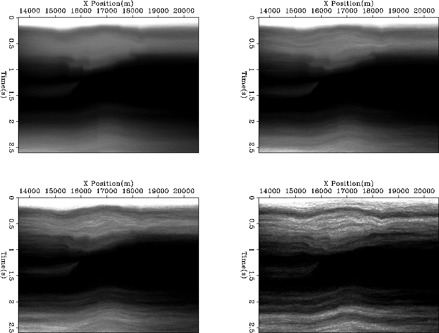
To test the methodology I took a 2-D line from a 3-D North Sea dataset provided by Unocal. Figure  shows four different realizations with varying levels of $\sigma$.

 

scale.10.x2
Figure 9 Four different realization of fitting goals (12) with increasing levels of Gaussian noise in $\bf v$.

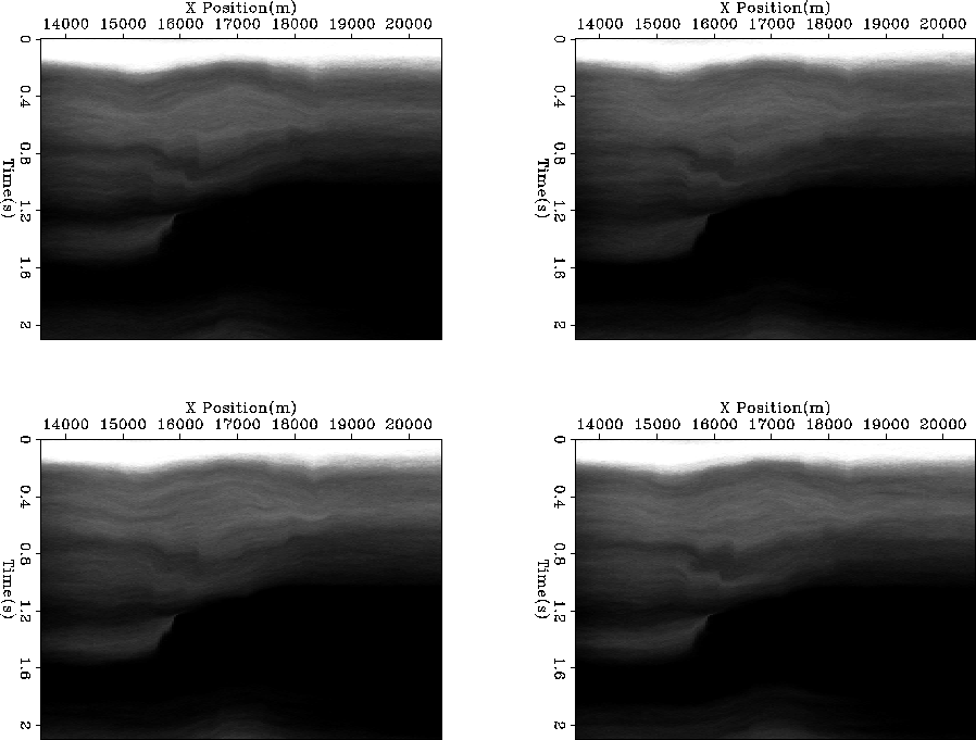
I then chose what I considered a reasonable variability level, and constructed ten equiprobable models (Figure ). Note that the general shapes of the models are very similar. What we see are smaller structural changes. For example, look at the range between .7s and 1.1s. Generally each realization tries to put a high velocity layer in this region, but thickness and magnitude varies in the different realizations.

 

dix-real
Figure 10 Four of the ten different realization of fitting goals (12) with constant Gaussian noise in $\bf v$.