Examples

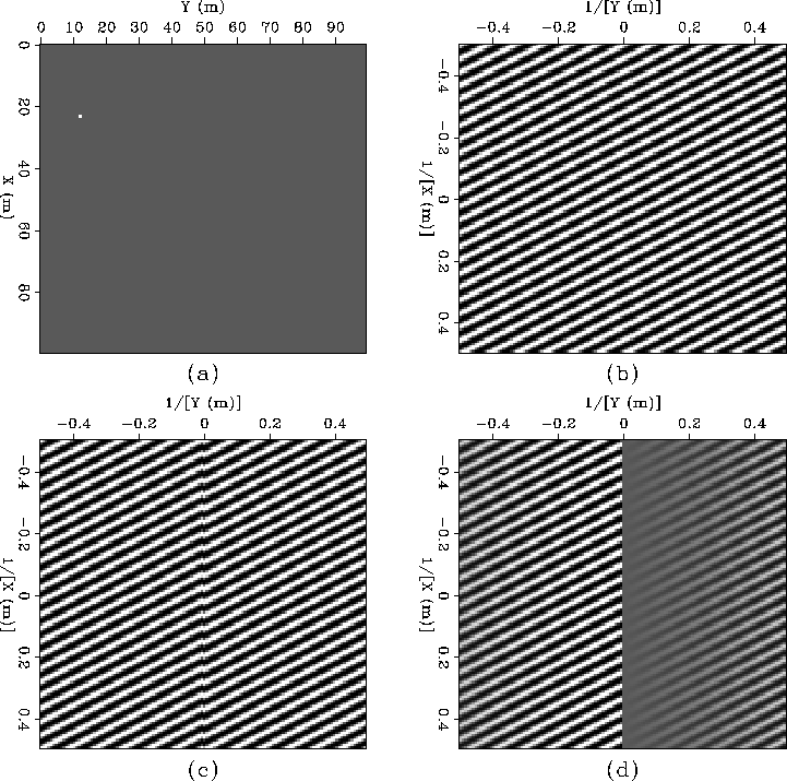
Figure 4 compares the real part of the 2-D Fourier transform of a single spike with the equivalent real part after a 1-D FFT in helical boundary conditions. The Fourier transforms are centered, so that zero frequency is at the center of the plot. This has the effect that the artifacts that would appear at the vertical boundaries (k_y=0) of the image are more visible since they appear at the center of the plot.

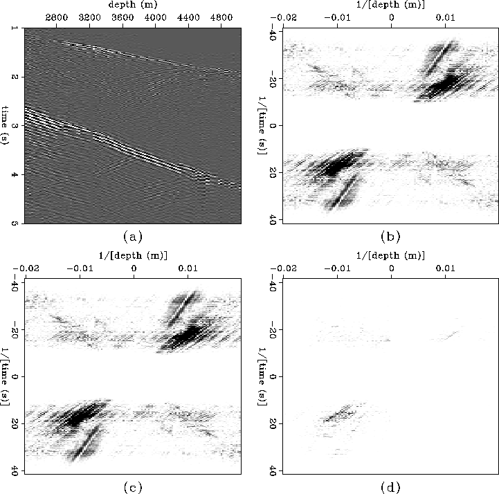
Figure 5 compares amplitude spectra for a broader band 2-D seismic VSP gather. Artifacts from the helical boundaries are very difficult to see on the spectra themselves, and the difference image is very low amplitude.

 

spikespec
Figure 4 Comparison of real part of 2-D spectra: (a) input spike (single frequency), (b) real part of 2-D FFT, (c) real part of 1-D helical FFT, and (d) difference between (b) and (c) clipped to same level.

 

schlumspec
Figure 5 Comparison of 2-D amplitude spectra: (a) input 2-D VSP gather, (b) amplitude spectrum from 2-D FFT, (c) amplitude spectrum from 1-D helical FFT, and (d) difference between (b) and (c) clipped to same level.