Signal and noise separation

Signal and noise separation and noise attenuation are yet another important application of plane-wave prediction filters Abma (1995); Brown et al. (1999); Canales (1984); Claerbout and Fomel (2000); Clapp and Brown (2000); Soubaras (1995); Spitz (1999).

The problem has a very clear interpretation in terms of the local dip components. If two components, $\bold{s}_1$ and $\bold{s}_2$ are estimated from the data, and we can interpret the first component as signal, and the second component as noise, then the signal and noise separation problem reduces to solving the least-squares system

$$\begin{eqnarray} \bold{C}(\bold{s}_1) \bold{d}_1 & \approx & 0 \;, \ \epsilon \bold{C}(\bold{s}_2) \bold{d}_2 & \approx & 0 \;\end{eqnarray}$$ (19) (20)

for the unknown signal and noise components $\bold{d}_1$ and $\bold{d}_2$ of the input data $\bold{d}$: 

$$\bold{d}_1 + \bold{d}_2 = \bold{d}.$$ (21)

The scalar parameter $\epsilon$ in equation (20) reflects the signal to noise ratio. We can combine equations (19-20) and (21) in the explicit system for the noise component $\bold{d}_2$:

$$\begin{eqnarray} \bold{C}(\bold{s}_1) \bold{d}_2 & \approx & \bold{C}(\bold{s... ...\;, \ \epsilon \bold{C}(\bold{s}_2) \bold{d}_2 & \approx & 0 \;.\end{eqnarray}$$ (22) (23)

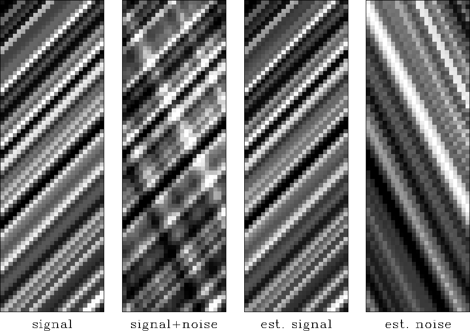
Figure 17 shows a simple example of the described approach. I estimated two dip components from the input synthetic data in a manner similar to that of Figure 10, and separated the corresponding events by solving the least-squares system (22-23). The separation result is visually perfect.

 

sn2
Figure 17 Simple example of dip-based single and noise separation. From left to right: ideal signal, input data, estimated signal, estimated noise.

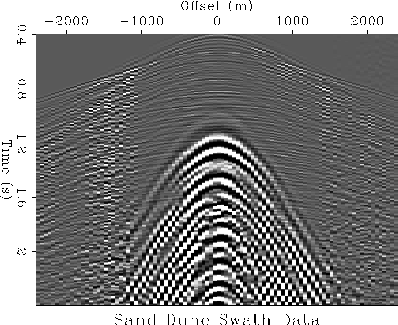
Figure 18 presents a significantly more complicated case: a receiver line from of a 3-D land shot gather from Saudi Arabia, contaminated with three-dimensional hyperbolic ground-roll. The same dataset has been used previously by Brown et al. (1999). The ground-roll noise and the reflection events have a significantly different frequency content, which might suggest an idea of separating them on the base of frequency alone. The result of frequency-based separation, shown in Figure 19 is, however, not ideal: part of the noise remains in the estimated signal after the separation. Changing the $\epsilon$ parameter in equation (23) could clean up the signal estimate, but it would also bring some of the signal into the subtracted noise. A better strategy is to separate the events by using both the difference in frequency and the difference in slope. For that purpose, I adopted the following algorithm:

1.

Use a frequency-based separation (or, alternatively, a simple low-pass filtering) to obtain an initial estimate of the ground-roll noise.

2.

Select a window around the initial noise. The further separation will happen only in that window.

3.

Estimate the noise dip from the initial noise estimate.

4.

Estimate the signal dip in the selected data window as the complimentary dip component to the already known noise dip.

5.

Use the signal and noise dips together with the signal and noise frequencies to perform the final separation. This is achieved by cascading single-dip plane-wave destructor filters with local 1-D three-coefficient PEFs, destructing a particular frequency.

The separation result is shown in Figure 20. The separation goal has been fully achieved: the estimated ground-roll noise is free of the signal components, and the estimated signal is free of the noise.

 

dune-dat
Figure 18 Ground-roll-contaminated data from Saudi Arabian sand dunes. A slice out of a 3-D shot gather.

 

dune-exp
Figure 19 Signal and noise separation based on frequency. Top: estimated signal. Bottom: estimated noise.

 

dune-sn
Figure 20 Signal and noise separation based on both dip and frequency. Top: estimated signal. Bottom: estimated noise.

The left plot in Figure 21 shows another test example: a shot gather contaminated by nearly linear low-velocity noise. In this case, a simple dip-based separation was sufficient for achieving a good result. The algorithm proceeds as follows

1.

Bandpass the original data with an appropriate low-pass filter to obtain an initial noise estimate (the right plot in Figure 21.)

2.

Estimate the local noise dip from the initial noise model.

3.

Estimate the signal dip from the input data as the complimentary dip component to the already known noise dip.

4.

Estimate the noise by an iterative optimization of system (22-23) and subtract it from the data to get the signal estimate.

Figure 22 shows the separation result. The signal and noise components are nicely separated. Guitton (2000) uses the same data example to develop a method of pairing noise separation with stacking velocity analysis.

 

ant-dat
Figure 21 Left: Input noise-contaminated shot gather. Right: Result of low-pass filtering.

 

ant-sn
Figure 22 Signal and noise separation based on dip. Left: estimated signal. Right: estimated noise.

The examples in this subsection show that when the signal and noise components have distinctly different local slopes, we can successfully separate them with plane-wave destructor filters.