Representing covariance matrices by sparse operators

In order to understand the structure of the matrices $\bold{C}_{md}$and $\bold{C}_d$, we need to make some assumptions about the relationship between the true model $\bold{m}$ and the data $\bold{d}$. A natural assumption is that if the model were known exactly, the observed data would be related to it by a forward interpolation operator $\bold{L}$ as follows:  

$$\bold{d} = \bold{L}\,\bold{m} + \bold{n}\;,$$ (4)

where $\bold{n}$ is an additive observational noise. For simplicity, we can assume that the noise is uncorrelated and normally distributed around zero:  

$$\bold{C}_{mn} = 0\;;\quad\bold{C}_n = \sigma_n^2\,\bold{I}\;,$$ (5)

where $\bold{I}$ is an identity matrix of the data size, and $\sigma_n$ is a scalar. Assuming that there is no linear correlation between the noise and the model, we arrive at the following expressions for the second moment matrices in formula ():  

$$\bold{C}_{d} = E\left[\left(\bold{L}\,\bold{m} + \bold{n}\r... ...= \bold{L}\,\bold{C}_{m}\,\bold{L}^T + \sigma_n^2\,\bold{I}\;,$$ (6)

 

$$\bold{C}_{md} = E\left[\bold{m}\, \left(\bold{m}^T\,\bold{L}^T + \bold{n}^T\right)\right] = \bold{C}_{m}\,\bold{L}^T\;.$$ (7)

Substituting equations () and () into (), we finally obtain the following specialized form of the Gauss-Markoff formula:  

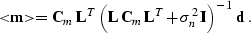$$<\!\!\bold{m}\!\!\gt = \bold{C}_{m}\,\bold{L}^T\,\left( \b... ...\,\bold{L}^T + \sigma_n^2\,\bold{I}\right)^{-1}\, \bold{d}\;.$$ (8)

Assuming that $\bold{C}_{m}$ is invertible, we can also rewrite equation () in a mathematically equivalent form  

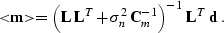$$<\!\!\bold{m}\!\!\gt = \left(\bold{L}\,\bold{L}^T + \sigma_n^2\,\bold{C}_m^{-1}\right)^{-1}\,\bold{L}^T\,\bold{d}\;.$$ (9)

The equivalence of formulas () and () follows from the simple matrix equality  

$$\bold{C}_m \bold{L}^T (\bold{L} \bold{C}_m \bold{L}^T + \sig... ...L}^T \bold{L} + \sigma_n^2 \bold{C}_m^{-1})^{-1} \bold{L}^T\;.$$ (10)

It is important to note an important difference between equations () and (): The inverted matrix has data dimensions in the first case, and model dimensions in the second case. I discuss the practical significance of this distinction in Chapter .

In order to simplify the model estimation problem further, we can introduce a local differential operator $\bold{D}$. A model $\bold{m}$complies with the operator $\bold{D}$ if the residual after we apply this operator $\bold{r} = \bold{D}\,\bold{m}$ is uncorrelated and normally distributed. This means that  

$$E\left[\bold{D}\,\bold{m}\,\bold{m}^T\,\bold{D}^T\right] = \bold{D}\,\bold{C}_m\,\bold{D}^T = \sigma_m^2\,\bold{I}\;,$$ (11)

where the identity matrix $\bold{I}$ has the model size. Furthermore, assuming that $\bold{D}$ is invertible, we can represent $\bold{C}_{m}$as follows:  

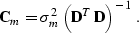$$\bold{C}_m = \sigma_m^2\,\left(\bold{D}^T\,\bold{D}\right)^{-1}\;.$$ (12)

Substituting formula () into () and (), we can finally represent the model estimate in the following equivalent forms:

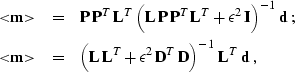$$\begin{eqnarray} <\!\!\bold{m}\!\!\gt & = & \bold{P}\,\bold{P}^T\,\bold{L}^T\,\... ...silon^2\,\bold{D}^T\,\bold{D}\right)^{-1}\,\bold{L}^T\,\bold{d}\;,\end{eqnarray}$$ (13) (14)

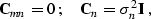
where 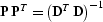$\bold{P}\,\bold{P}^T = \left(\bold{D}^T\,\bold{D}\right)^{-1}$and $\epsilon = \frac{\sigma_n}{\sigma_m}$.

The first simplification step has now been accomplished. By introducing additional assumptions, we have approximated the covariance matrices $\bold{C}_d$ and $\bold{C}_{md}$ with the forward interpolation operator $\bold{L}$ and the differential operator $\bold{D}$. Both $\bold{L}$ and $\bold{D}$ act locally on the model. Therefore, they are sparse, efficiently computed operators. Different examples of operators $\bold{L}$, $\bold{D}$, and $\bold{P}$ are discussed later in this dissertation. In the next section, I proceed to the second simplification step.