

Next: Two-dimensional environmental data examples
Up: Wilson-Burg spectral factorization
Previous: Comparison of Wilson-Burg and
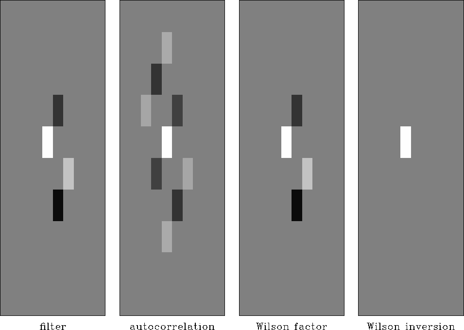
The first simple example of helical spectral factorization is shown in
Figure ![[*]](http://sepwww.stanford.edu/latex2html/cross_ref_motif.gif) . A minimum-phase factor is found by
spectral factorization of its autocorrelation. The result is
additionally confirmed by applying inverse recursive filtering, which
turns the filter into a spike (the rightmost plot in
Figure
. A minimum-phase factor is found by
spectral factorization of its autocorrelation. The result is
additionally confirmed by applying inverse recursive filtering, which
turns the filter into a spike (the rightmost plot in
Figure ![[*]](http://sepwww.stanford.edu/latex2html/cross_ref_motif.gif) .)
.)
autowaves
Figure 12 Example of 2-D Wilson-Burg
factorization. From left to right: the input filter; its
auto-correlation; the factor obtained by the Wilson-Burg method; the
result of the deconvolution.


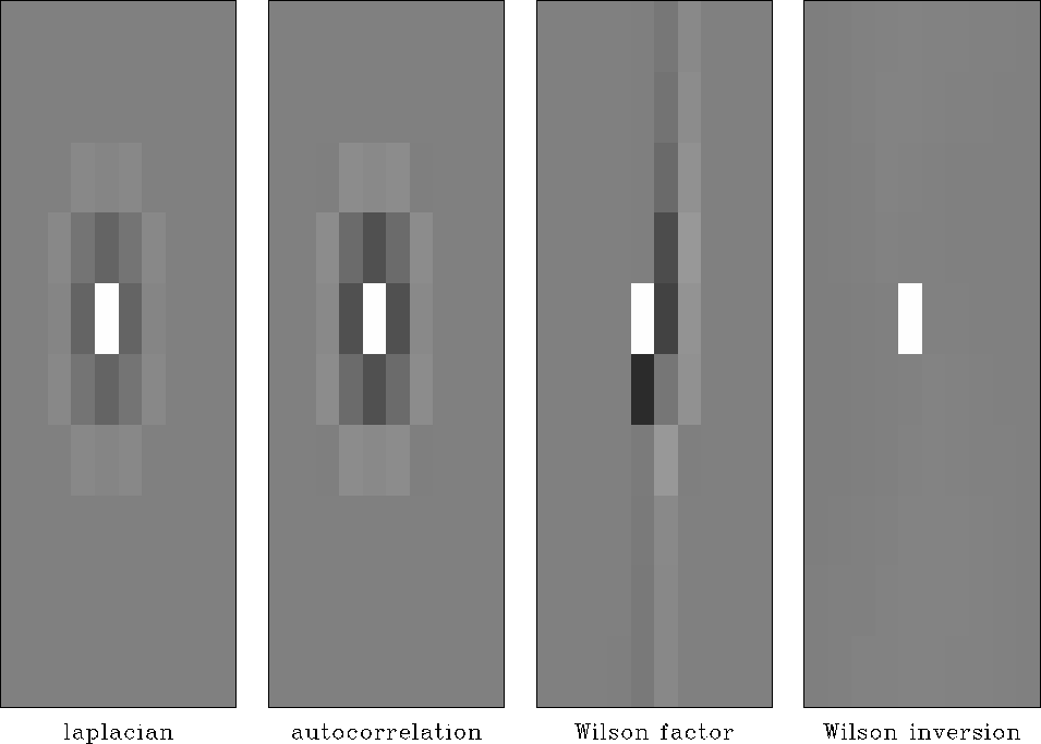
A practically useful example is depicted in Figure ![[*]](http://sepwww.stanford.edu/latex2html/cross_ref_motif.gif) .
The symmetric Laplacian operator is often used in practice for
regularizing smooth data (see a more detailed discussion in
Chapter
.
The symmetric Laplacian operator is often used in practice for
regularizing smooth data (see a more detailed discussion in
Chapter ![[*]](http://sepwww.stanford.edu/latex2html/cross_ref_motif.gif) ). In order to construct a corresponding
recursive preconditioner, I factor the Laplacian auto-correlation (the
biharmonic operator) using the Wilson-Burg algorithm.
Figure
). In order to construct a corresponding
recursive preconditioner, I factor the Laplacian auto-correlation (the
biharmonic operator) using the Wilson-Burg algorithm.
Figure ![[*]](http://sepwww.stanford.edu/latex2html/cross_ref_motif.gif) shows the resultant filter. The minimum-phase
Laplacian filter has several times more coefficients that the original
Laplacian. Therefore, its application would be more expensive in a
convolution application. The real advantage follows from the
applicability of the minimum-phase filter for inverse filtering
(deconvolution). As demonstrated by 2-D examples later in this
chapter, the gain in convergence from recursive filter preconditioning
outweighs the loss of efficiency from the longer filter.
Figure
shows the resultant filter. The minimum-phase
Laplacian filter has several times more coefficients that the original
Laplacian. Therefore, its application would be more expensive in a
convolution application. The real advantage follows from the
applicability of the minimum-phase filter for inverse filtering
(deconvolution). As demonstrated by 2-D examples later in this
chapter, the gain in convergence from recursive filter preconditioning
outweighs the loss of efficiency from the longer filter.
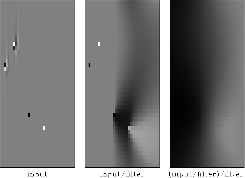
Figure ![[*]](http://sepwww.stanford.edu/latex2html/cross_ref_motif.gif) shows a construction of the smooth inverse
impulse response by application of the
shows a construction of the smooth inverse
impulse response by application of the  operator, where
  is deconvolution with the minimum-phase
Laplacian. The application of
  is equivalent to a numerical
solution of the biharmonic equation, discussed in
Chapter
 ![[*]](http://sepwww.stanford.edu/latex2html/cross_ref_motif.gif) .
.
laplac
Figure 13 Creating a minimum-phase
Laplacian filter. From left to right: Laplacian filter; its
auto-correlation; the factor obtained by the Wilson-Burg method
(minimum-phase Laplacian); the result of the deconvolution.


 thin42
Figure 14 2-D deconvolution with the
minimum-phase Laplacian. Left: input. Center: output of
deconvolution. Right: output of deconvolution and adjoint
deconvolution (equivalent to solving the biharmonic differential
equation).


Next: Two-dimensional environmental data examples
Up: Wilson-Burg spectral factorization
Previous: Comparison of Wilson-Burg and
Stanford Exploration Project
12/28/2000
![[*]](http://sepwww.stanford.edu/latex2html/cross_ref_motif.gif) . A minimum-phase factor is found by
spectral factorization of its autocorrelation. The result is
additionally confirmed by applying inverse recursive filtering, which
turns the filter into a spike (the rightmost plot in
Figure
. A minimum-phase factor is found by
spectral factorization of its autocorrelation. The result is
additionally confirmed by applying inverse recursive filtering, which
turns the filter into a spike (the rightmost plot in
Figure ![[*]](http://sepwww.stanford.edu/latex2html/cross_ref_motif.gif) .)
.)

![[*]](http://sepwww.stanford.edu/latex2html/cross_ref_motif.gif) .
The symmetric Laplacian operator is often used in practice for
regularizing smooth data (see a more detailed discussion in
Chapter
.
The symmetric Laplacian operator is often used in practice for
regularizing smooth data (see a more detailed discussion in
Chapter ![[*]](http://sepwww.stanford.edu/latex2html/cross_ref_motif.gif) ). In order to construct a corresponding
recursive preconditioner, I factor the Laplacian auto-correlation (the
biharmonic operator) using the Wilson-Burg algorithm.
Figure
). In order to construct a corresponding
recursive preconditioner, I factor the Laplacian auto-correlation (the
biharmonic operator) using the Wilson-Burg algorithm.
Figure ![[*]](http://sepwww.stanford.edu/latex2html/cross_ref_motif.gif) shows the resultant filter. The minimum-phase
Laplacian filter has several times more coefficients that the original
Laplacian. Therefore, its application would be more expensive in a
convolution application. The real advantage follows from the
applicability of the minimum-phase filter for inverse filtering
(deconvolution). As demonstrated by 2-D examples later in this
chapter, the gain in convergence from recursive filter preconditioning
outweighs the loss of efficiency from the longer filter.
Figure
shows the resultant filter. The minimum-phase
Laplacian filter has several times more coefficients that the original
Laplacian. Therefore, its application would be more expensive in a
convolution application. The real advantage follows from the
applicability of the minimum-phase filter for inverse filtering
(deconvolution). As demonstrated by 2-D examples later in this
chapter, the gain in convergence from recursive filter preconditioning
outweighs the loss of efficiency from the longer filter.
Figure ![[*]](http://sepwww.stanford.edu/latex2html/cross_ref_motif.gif) shows a construction of the smooth inverse
impulse response by application of the
shows a construction of the smooth inverse
impulse response by application of the ![]() operator, where
operator, where ![]() is deconvolution with the minimum-phase
Laplacian. The application of
is deconvolution with the minimum-phase
Laplacian. The application of ![]() is equivalent to a numerical
solution of the biharmonic equation, discussed in
Chapter
is equivalent to a numerical
solution of the biharmonic equation, discussed in
Chapter ![[*]](http://sepwww.stanford.edu/latex2html/cross_ref_motif.gif) .
.

