


The general method of B-spline regularization, outlined in
Chapter ![[*]](http://sepwww.stanford.edu/latex2html/cross_ref_motif.gif) , is easily applicable for the case of
local plane-wave destruction. The continuous regularization operator
D in this case comes from the theoretical plane-wave differential
equation (). We simply need to construct the
auto-correlation filter dj according to formula () and
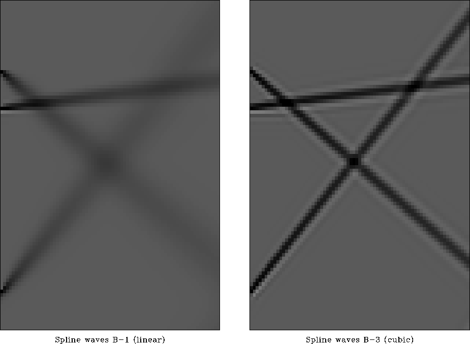
factorize it with the Wilson-Burg method. Figure
shows three plane waves constructed from three distant spikes by
application of inverse recursive filtering with two different B-spline
regularizers. The left plot was obtained with first-order B-splines
(equivalent to linear interpolation). This type of regularizer is
identical to Clapp's steering filters Clapp et al. (1997) and
suffers from numerical dispersion effects. The right plot was obtained
with third-order splines. Most of the dispersion is suppressed by
using a more accurate interpolation.
, is easily applicable for the case of
local plane-wave destruction. The continuous regularization operator
D in this case comes from the theoretical plane-wave differential
equation (). We simply need to construct the
auto-correlation filter dj according to formula () and
factorize it with the Wilson-Burg method. Figure
shows three plane waves constructed from three distant spikes by
application of inverse recursive filtering with two different B-spline
regularizers. The left plot was obtained with first-order B-splines
(equivalent to linear interpolation). This type of regularizer is
identical to Clapp's steering filters Clapp et al. (1997) and
suffers from numerical dispersion effects. The right plot was obtained
with third-order splines. Most of the dispersion is suppressed by
using a more accurate interpolation.
 |
![[*]](http://sepwww.stanford.edu/latex2html/movie.gif)


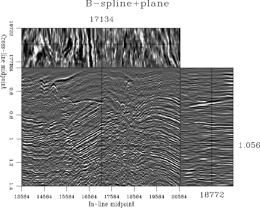
Equipped with the powerful B-spline plane-wave construction, we can
now approach the main goal of this work: three-dimensional seismic
data regularization. For an illustrative test, I chose the North Sea
dataset, which was previously used for testing azimuth moveout
Biondi et al. (1998) and common-azimuth migration
Biondi (1996). Figure in the introduction
showed the highly irregular midpoint geometry for a selected in-line
and cross-line offset bin in the data. The data irregularity is also
evident in the bin fold map, shown in Figure . The
goal of data regularization is to create a regular data cube at the
specified bins from the irregular input data, which have been
preprocessed by normal moveout.
|
fold-win
Figure 19 Map of the fold distribution for the 3-D data test. | 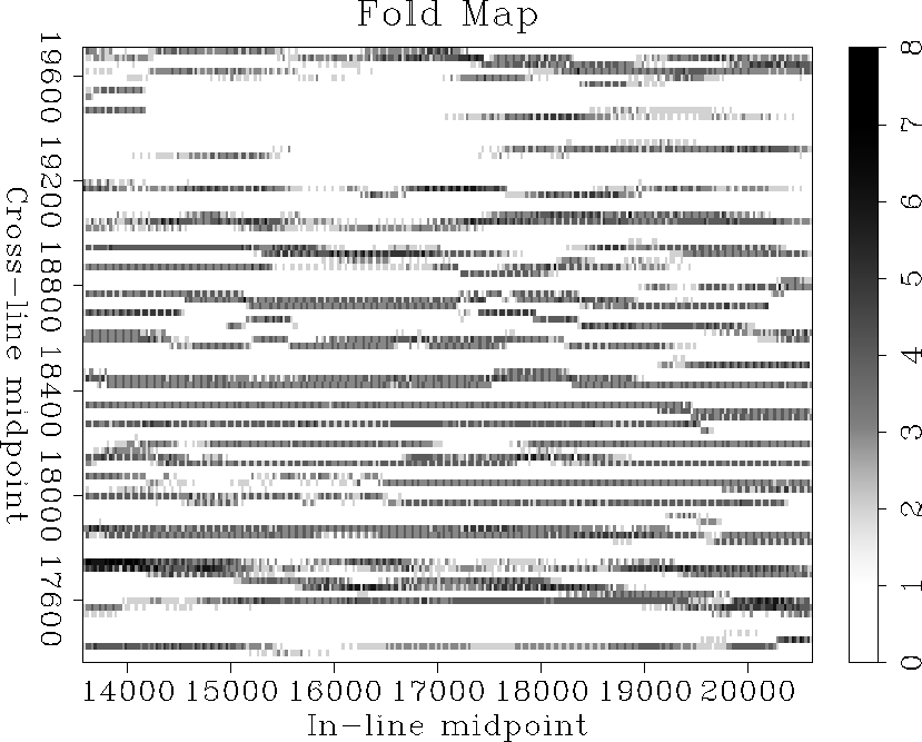 |
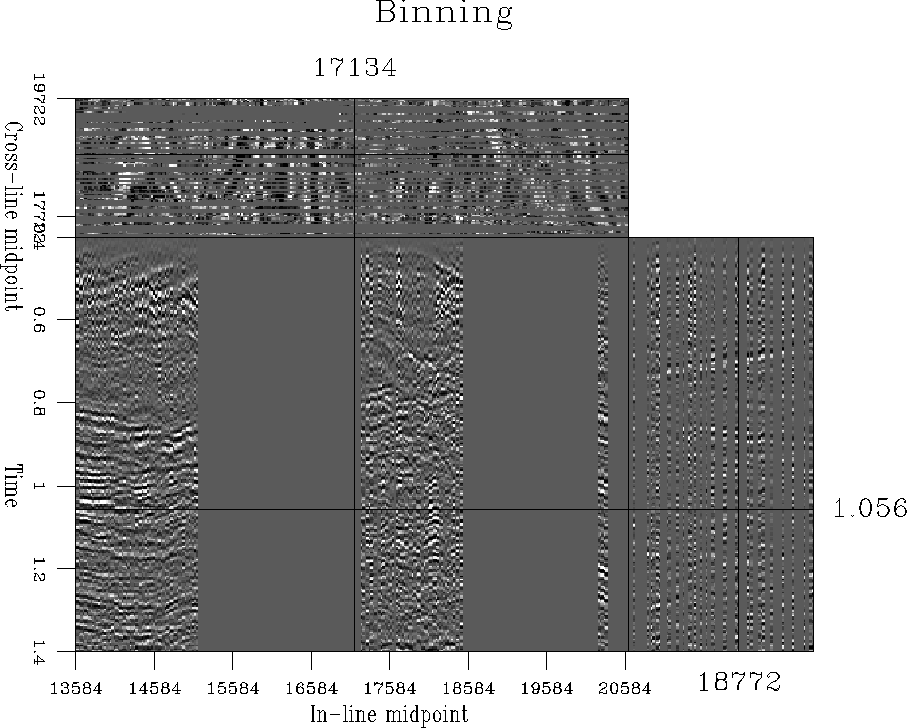
The data cube after normalized binning is shown in
Figure . Binning works reasonably well in the areas of
large fold but fails to fill the zero fold gaps and has an overall
limited accuracy.
 |
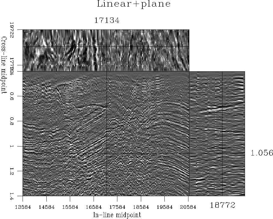
For efficiency, I perform regularization on individual time slices.
Figure shows the result of regularization using
bi-linear interpolation and smoothing preconditioning with the
minimum-phase Laplacian filter. The empty bins are filled in a
consistent manner but the data quality is distorted because simple
smoothing fails to characterize the complicated data structure.
Instead of continuous events, we see smoothed blobs in the time
slices. The events in the in-line and cross-line sections are also not
clearly pronounced.
 |
We can use the smoothing regularization result to estimate the local
dips in the data, design invertible local plane-wave destruction
filters, and repeat the regularization process. Inverse interpolation
using bi-linear interpolations with plane-wave preconditioning is
shown in Figure . The regularization result is
improved: the continuous reflection events become clearly visible in
the time slices. As expected, a higher quality result is achieved with
cubic B-spline (Figure ). Regularization works
again in constant time slices, using recursive filter preconditioning
with plane-wave destructor filters analogous to those in
Figure . Despite the irregularities in the input data,
the regularization result preserves both flat reflection events and
steeply-dipping diffractions. Preserving diffractions is important for
correct imaging of sharp edges in the subsurface structure
Biondi and Palacharla (1996b).
For simplicity, I assumed only a single local dip component in the
data. This assumption degrades the result in the areas of multiple
conflicting dips, such as the intersections of plane reflections and
hyperbolic diffractions in Figure . One could
improve the regularization result by considering multiple local dips.
In the next section of this chapter, I describe an alternative
offset-continuation approach, which uses a physical connection between
neighboring offsets instead of assuming local continuity in the
midpoint domain.
 |
 |
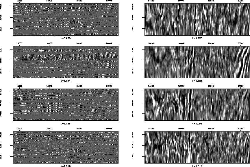
The 3-D results of this subsection were obtained with an efficient 2-D
regularization in time slices. This approach is computationally
attractive because of its easy parallelization: different slices can
be interpolated independently and in parallel.
Figure shows the interpolation result for four
selected time slices. Local plane waves, barely identifiable after
binning (left plots in Figure ), appear clear and
continuous in the interpolation result (right plots in
Figure ). Different time slices are assembled
together to form the 3-D cube shown in Figure .
A more powerful, although less convenient, approach to 3-D data regularization, is the full 3-D plane-wave destruction. I discuss it in the next subsection.
 |