Operator antialiasing and least-squares inversion

The PRT in the Fourier domain allows us to derive a least-squares estimate of the data in the radon domain. Equations (7) and (8) suggest the use of inversion to recover the original amplitude in the data. In computing the pseudo-inverse of the matrix ${\bf L}$, two cases need to be distinguished.

The under-determined case: The least-squares inverse of m for each frequency is  

$${\bf \hat{m}_{under}} = {\bf L'}({\bf LL'}+\epsilon{\bf I})^{-1}{\bf d},$$ (14)

where ${\bf \hat{m}}$ is the estimate of the model, ${\bf LL'+ \epsilon{\bf I}}$ a matrix $nx\times nx$ to invert, and $\epsilon = \sigma_d^2/\sigma_m^2$.

The over-determined case: The least-squares inverse for m for each frequency is  

$${\bf \hat{m}_{over}} = ({\bf L'L}+\epsilon{\bf I})^{-1}{\bf L'd},$$ (15)

where ${\bf L'L+}\epsilon{\bf I}$ is a $nq\times nq$ matrix to invert with a Toeplitz structure Darche (1990); Kostov (1989).

An interesting problem occurs when the conditioning of the matrix quickly deteriorates as frequencies increase. This effect is partly caused by the frequency truncation of the operator. A solution to this problem is to increase $\epsilon$, which appears in equations (14) and (15), with the frequency. To do so, I set  

$$\epsilon_{\omega} = \mbox{log}(n_w+1)*\beta,$$ (16)

where n_w is the index of the computing frequency and $\beta$ a constant to set apriori. This choice of $\epsilon_{\omega}$ allows us to increase the regularization with the frequency but not too much. Indeed a too strong regularization would affect the amplitude recovery of the data.

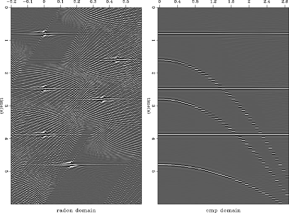
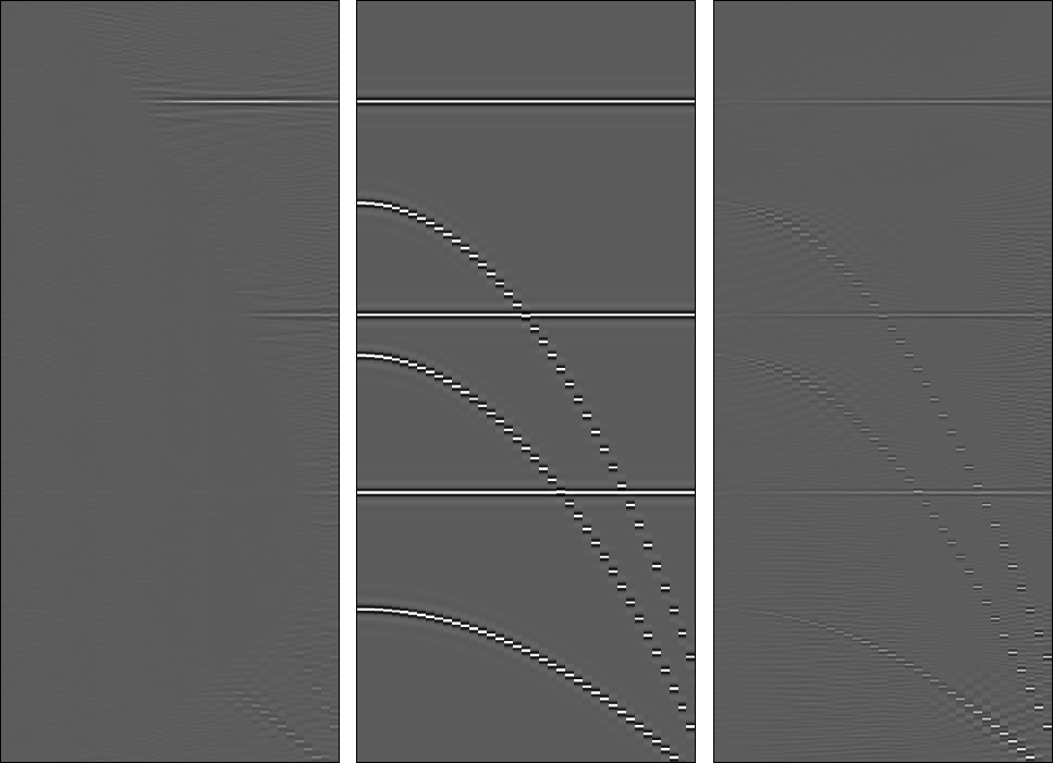
The size of the matrix to invert makes possible the use of direct inversion as opposed to iterative processes. Figure 5 shows the result of inversion using the aliased operator. The aliasing artifacts are still strong, but some energy has focused, decreasing the width of the horizontal events caused by near-offset aperture effects. The resulting data, which appear in the right panel of Figure 5, are almost perfectly recovered. The residual in the left panel of Figure 7 demonstrates that the data fitting is nearly perfect.

 

inval
Figure 5 Left: The parabolic radon domain after least-squares inversion. The events of interest are more focused, but the aliasing artifacts remain. Right: The reconstructed data; the result is nearly perfect.

Now, using the antialiasing conditions on the operator, we obtain the data in Figure 6: events are better focused in the radon domain and most of data aliasing artifacts have disappeared. We observe a loss of resolution for the non-flat events caused by the antialiasing conditions. The aliasing of the input data produces the remaining noisy events in the radon domain. Again, the data in the right panel of Figure 6 are almost completely recovered, and the residual in the right panel of Figure 7 is very small.

 

invna
Figure 6 Left: The parabolic radon domain after inversion of the antialiasing operator. The events are more focused and the aliasing artifacts have been weakened. We see a loss of resolution caused by the antialiasing conditions. The aliasing of the input data produces the remaining noisy events. Right: The reconstructed data.

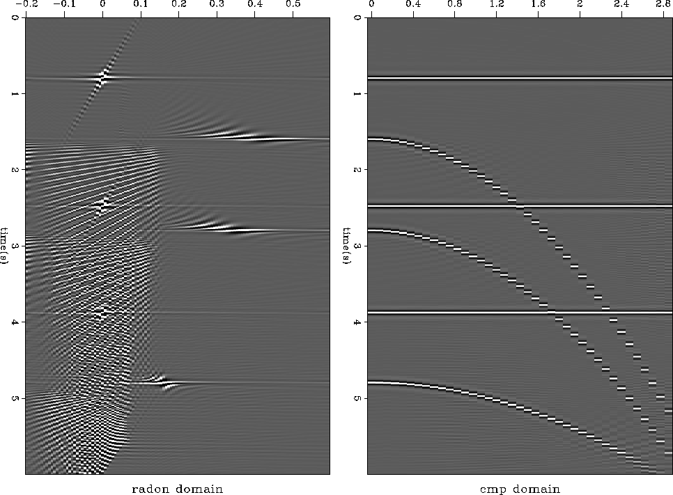This result proves that the antialiasing PRT can be inverted as long as $\epsilon$ is provided. It also proves that the use of antialiasing conditions on the operator helps to mitigate data aliasing artifacts. However, as Figure 6 indicates, data aliasing effects can't be totally removed. The next section shows that sparseness conditions in the radon domain can destroy data aliasing artifacts.

 

comp
Figure 7 Left: Residual for the aliased operator with least-squares inversion. Middle: Input data. Right: Residual for the antialiasing operator with least-squares inversion.