Numerical comparison

The Amoco 2.5-D synthetic dataset Etgen and Regone (1998) provides an excellent test for the weighting functions discussed above.

The velocity model (Figure 1) contains significant structural complexity in the upper 3.8 km, and a flat reflector of uniform amplitude at about 3.9 km depth. Since the entire velocity model (``Canadian foothills overthrusting onto the North Sea'') is somewhat pathological, I restricted my experiments to the North Sea section of the dataset (x>10 km). The data were generated by 3-D acoustic finite-difference modeling of the 2.5-D velocity model. However, making the test more difficult is the fact that the 2-D linear one-way recursive extrapolators Ristow and Ruhl (1994) that I use for modeling and migration do not accurately predict the 3-D geometric spreading and multiple reflections that are present in this dataset.

 

amocovel
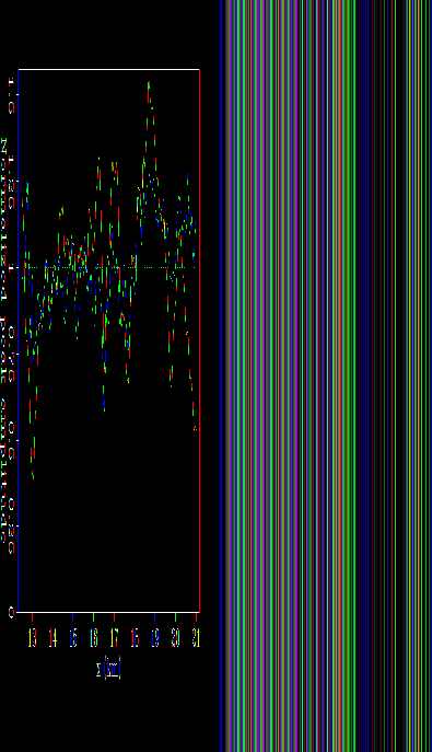
Figure 1 Velocity (in km/s) model used to generate the synthetic Amoco 2.5-D dataset.

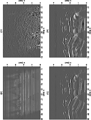
Figure 2 compares the migrated image (${\bf m}_1$)with the results of remodeling and remigrating the three reference images described above. The imprint of the recording geometry is clearly visible on the three remigrations in Figures 2 (b-d).

Figure 3 compares the illumination calculated from the three reference images with the raw shot illumination. Noticably, the shot-only weighting function [panel (a)] does not take into account the off-end (as opposed to split-spread) receiver geometry. Panel (b), the weighting function derived from model ${\bf m}_1$, appears slightly noisy. However, in well-imaged areas (e.g. along the target reflector), the weighting function is well-behaved. Panel (c) shows the weighting function derived from the random reference image (${\bf m}_2$). Despite the smoothing, this weighting function clearly bears the stamp of the random number field. A feature of white noise is that no amount of smoothing will be able to remove the effect of the random numbers completely. The final panel (d) shows the flat-event illumination weighting function, derived from ${\bf m}_3$. This is noise-free and very well-behaved since it depends only on the velocity model and recording geometry, not the data.

 

amocomigs
Figure 2 Comparison of calibration images: (a) original migration, (b) original migration after modeling and migration, (c) random image after modeling and migration, and (d) flat event image after modeling and migration.

 

amocowghts
Figure 3 Comparison of weighting functions: (a) original migration, (b) original migration after modeling and migration, (c) random image after modeling and migration, and (d) flat event image after modeling and migration.

For a quantitative comparison, I picked the maximum amplitude of the 3.9 s reflection event on the calibrated images. The normalized standard deviation (NSD) of these amplitudes is shown in Table 1, where

$$\mbox{NSD} = \sqrt{ \sum_{i_x} \left( \frac{a_{i_x}}{\bar a} - 1 \right )^2}.$$ (7)

Table 1, therefore, provides a measure of how well the various weighting function compensate for illumination difficulties. The amplitudes of the raw migration, and the migration after flat-event normalization are shown in Figure 4. This illustrates the numerical results from Table 1: for this model the normalization procedure improves amplitude reliability by almost a factor of two.

 

2||c|Weighting function: NSD:

2||c|No weighting function 0.229

2||c|Shot illumination 0.251

$${\bf m}_{\rm ref}={\bf m}_1$$ (migrated image) 0.148

$${\bf m}_{\rm ref}={\bf m}_2$$ (random image) 0.195

$${\bf m}_{\rm ref}={\bf m}_3$$ (flat events) 0.140

 

eventamp Figure 4 Normalized peak amplitude of 3.9 km reflector after migration (solid line), and then normalization by flat-event illumination (dashed line) derived with ${\bf m}_{\rm ref}={\bf m}_3$. The ideal result would be a constant amplitude of 1.