Results

Figure 1 shows a roughened image of the lake bottom constructed by using the three methods discussed above. All of the three models were computed with the same value of damping parameter ($\epsilon$) in a linear step of the IRLS iterations to make a fair comparison.

 

comp_1_ann
Figure 1 Comparison of the roughened results obtained by the three methods. Top: Result of IRLS with no residual whitener (system 2). Central: IRLS with a derivative operator as a residual whitener (system 3). Bottom: Our algorithm with a bank of PEFs as a residual whitener (system 4)

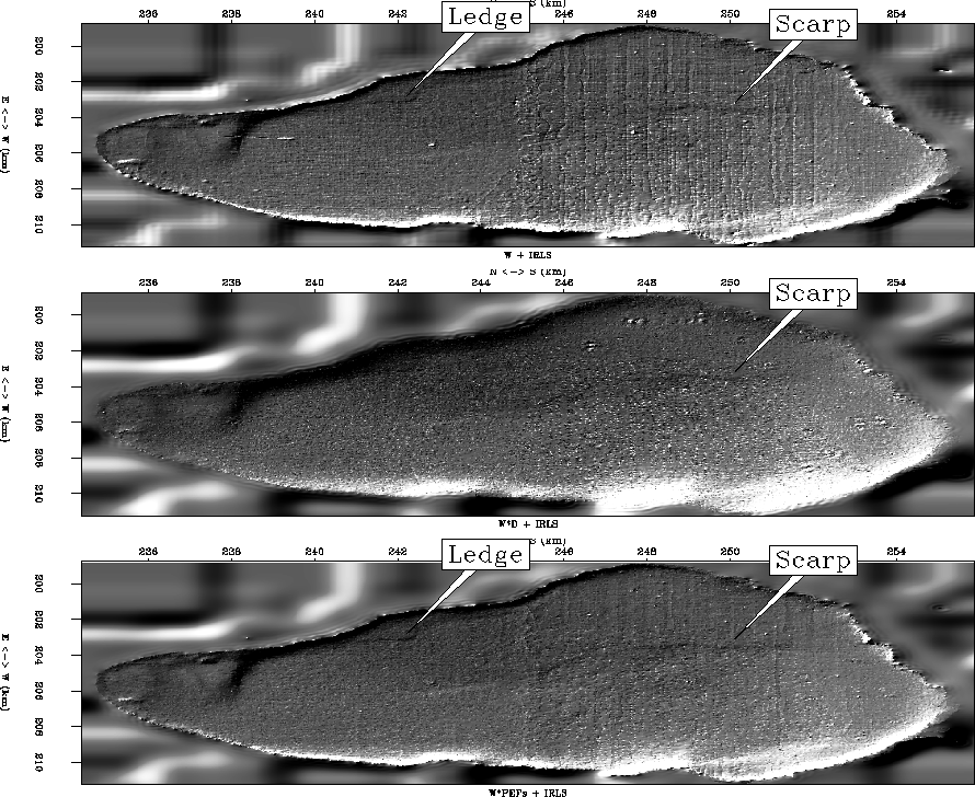The top panel of Figure 1 shows the result corresponding to system (2), implementing IRLS without whitening the residual. This panel has a strong acquisition footprint; some ``spikes'' are still present in the model, even though IRLS managed to attenuate most of them. At the same time this panel has a good resolution and we can see some fine features of the bottom, especially in the southern part of the lake where the acquisition footprint is weaker. The central panel of Figure 1 shows the result of solving system (3) with a derivative operator along the tracks as a residual whitener. This panel has no acquisition footprint but has a lower resolution as was observed by Fomel and Claerbout (1995). Although this method preserved main features of the bottom, some features such as a ledge marked in the image are not present in the model. The third panel presents the result of our algorithm. As we can see almost all of the ship's tracks and spikes are suppressed without a visible decrease in resolution. For example, the ledge we observed before is still present in the model. It is interesting to notice that the scarp is even easier to see here than in the first image, where it is obscured by the acquisition footprint.

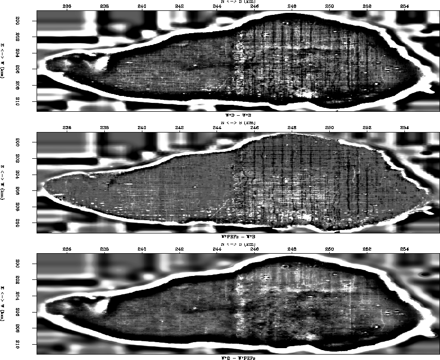
Figure 2 shows the difference among the results computed with the three algorithms discussed above.

The top panel shows the difference between the maps computed with IRLS without whitening the residual and IRLS with a derivative operator as a residual whitener. On this panel we can see ship tracks and features of the bottom which were attenuated from the final map. The central panel shows the difference between the maps computed with IRLS without whitening the residual and IRLS with a bank of PEFs as a residual whitener. Geological features are much less visible in this panel, but it is easy to see the acquisition footprint that our method removed. The third panel shows the difference between the final maps generated with the use of a derivative and a bank of PEFs to whiten the residual. On this panel we can still see some traces of the acquisition footprint which were left in the final map by our method. It is also easy to see the geological features of the bottom of the lake which were preserved by our method.

 

comp_2
Figure 2 Difference in the results obtained by the three methods. Top: Difference between IRLS without whitening the residual and with a derivative operator as a whitener. Central: Difference between IRLS without whitening the residual and IRLS with a bank of PEFs as a residual whitener. Bottom: Difference between IRLS with a derivative and a bank of PEFs as a whitener.