


| |
(1) |
| |
(2) |
![]()
| |
(3) |
![]()
With the above development of the Shuey equation, we see A is the normal incidence compressional reflection amplitude and B contains both normal incidence and angular dependence. Other authors, such as Castagna et al. (1998), have attempted to simplify this relationship by expressing B as a complicated function of A multiplied by new (empirical) fitting coefficients. While facilitating ever more cross-plotting possibilities, axes remain mixtures of compressional and shear quantities and yield little more insight.
However, with the above formulation of Shuey equation (1) we can
separate B into the compressional, A, and pseudo-shear, C, reflection
amplitude coefficients. Notice the very parallel structure
of the pseudo-shear, equation 3, to the normal
incidence term, equation 2, and its
independence from compressional velocity contrast. Encouragingly, the
pseudo-shear expression contracts to the normal incidence shear
reflection coefficient when the compressional to shear velocity ratio
![]() equals 2.
equals 2.
This separation (effectively between ![]() and
and ![]() ) will help guide our intuition by isolating the seismic reflection amplitude
into two components that have meaning in an AVA sense. Rather than
plotting on the
) will help guide our intuition by isolating the seismic reflection amplitude
into two components that have meaning in an AVA sense. Rather than
plotting on the ![]() plane, we can utilize the
plane, we can utilize the ![]() plane
and avoid an ordinate with codependency of compressional and shear
velocity boundary contrasts.
plane
and avoid an ordinate with codependency of compressional and shear
velocity boundary contrasts.
|
cartoon
Figure 1 With the clarity of structure of equation (3) for C, simple test case plots can be readily manufactured by applying it to mental scenarios within this cartoon. | 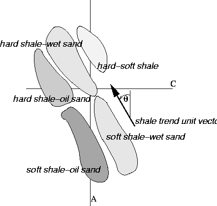 |

With the insight gained from the definitions of A and C, we can now intuitively understand that trends in this AVA plane are due to the variation of real rock properties. Figure 1 indicates the relative position of simple targets in this space. Because I have defined density and velocity as the properties of the lower layer, the negative values of A show a change from harder to softer intervals and the opposite is true for the positive values. Therefore we can understand something of the nature of the bounding layers of an interval as harder bounding lithologies will trend to more negative values of A.
We also
know that the shear velocity of a porous medium increases as we lower
the density of the included fluid. This tells us that the ![]() will be negative as we consider a water filled medium versus a gas
filled one and this will increasingly drive the value of C more
negative. The interplay between these compressional and shear
forces results in the normal NW-SE trend of the data cloud in Figure
1 indicating hard bounding rocks upward and soft ones downward.
will be negative as we consider a water filled medium versus a gas
filled one and this will increasingly drive the value of C more
negative. The interplay between these compressional and shear
forces results in the normal NW-SE trend of the data cloud in Figure
1 indicating hard bounding rocks upward and soft ones downward.
Gratwick (2001b) outlined the promise and difficulty of
prospecting AVA anomalies on an ![]() plane as explained by
Castagna and Swan (1997). Both authors stress the importance of the distance away
from the background trend for the analysis of a prospective event.
Attempting to quantify this, Gratwick (2001b)
calculates the product of A with B, then masks
the center mass of reflection amplitudes that are assumed to be
background values (non-prospective shale-wet sand or shale-shale
reflections). This process is shown in Figure 2.
The flaw in this method
is the dull spoon that differentiates anomalies from background. Not
only is the scalpel dull, but this methodology only appreciates a single
model type. More practically, the clumsy transfer in and out of SEP
architecture for graphical definition of the mute zone can dissuade
all but the most committed from utilizing this tool.
plane as explained by
Castagna and Swan (1997). Both authors stress the importance of the distance away
from the background trend for the analysis of a prospective event.
Attempting to quantify this, Gratwick (2001b)
calculates the product of A with B, then masks
the center mass of reflection amplitudes that are assumed to be
background values (non-prospective shale-wet sand or shale-shale
reflections). This process is shown in Figure 2.
The flaw in this method
is the dull spoon that differentiates anomalies from background. Not
only is the scalpel dull, but this methodology only appreciates a single
model type. More practically, the clumsy transfer in and out of SEP
architecture for graphical definition of the mute zone can dissuade
all but the most committed from utilizing this tool.
|
plot2
Figure 2 A vs. B scatter-plot with mute fairway defined. Gratwick (2001b) | 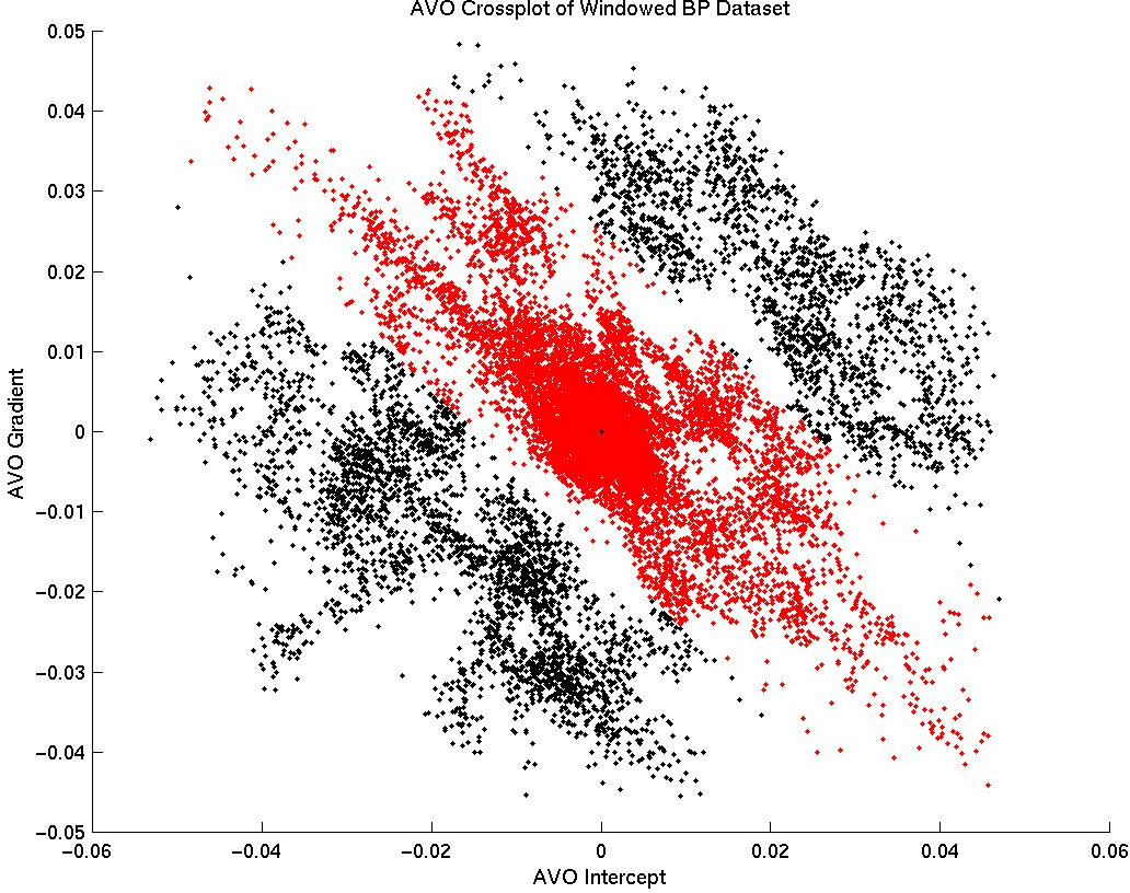 |
 |
![[*]](http://sepwww.stanford.edu/latex2html/movie.gif)


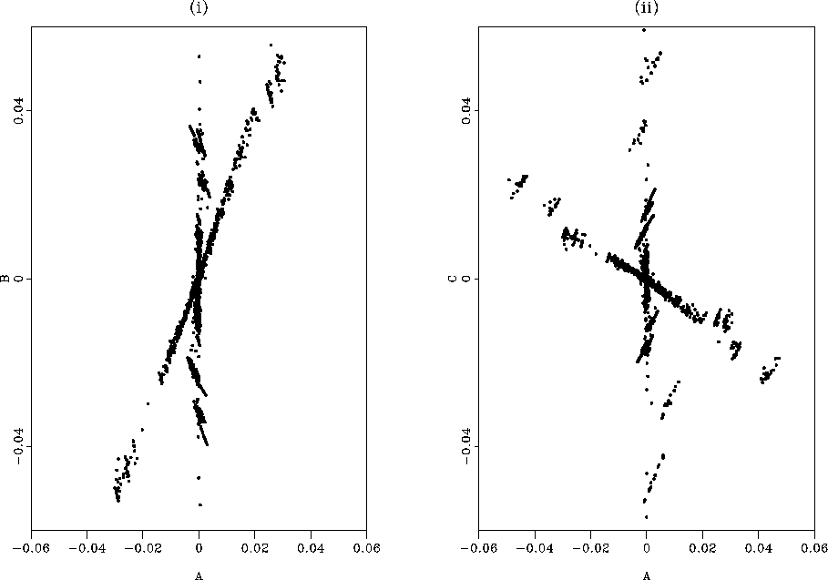
Figure 3 (i) shows the standard Slope-Intercept AVA
plot, while (ii) shows the transform to the Compressional-PseudoShear
plane. The data are generated from a synthetic provided by BP and
explained in detail by Gratwick (2001b). While immediately displeasing,
these two plots will highlight the power of the ![]() plane when
inspected. First note the strong zero presence on the intercept-axis
of the
plane when
inspected. First note the strong zero presence on the intercept-axis
of the ![]() panel. This is modeled data, boring, and makes our
unit vector for the shale trend very simple (
panel. This is modeled data, boring, and makes our
unit vector for the shale trend very simple (![]() ). In an
attempt to provide a small measure of
believable scatter (make this plot less boring), a bandpass
filter was run over the AVA attributes.
). In an
attempt to provide a small measure of
believable scatter (make this plot less boring), a bandpass
filter was run over the AVA attributes. ![[*]](http://sepwww.stanford.edu/latex2html/foot_motif.gif) This contributes to a few bothersome
artifacts, but are easy to neglect. These include: data present to the
left of shale trend (bandpassing returns negative values),
diagonal sub-trends of events, and incomplete orthogonalization. We see that due to the
presence of both shear and compressional velocity contrasts in the
formulation of B, the transition of reflections on the
This contributes to a few bothersome
artifacts, but are easy to neglect. These include: data present to the
left of shale trend (bandpassing returns negative values),
diagonal sub-trends of events, and incomplete orthogonalization. We see that due to the
presence of both shear and compressional velocity contrasts in the
formulation of B, the transition of reflections on the ![]() plot
from water to oil to gas takes place along a line with an acute angle
to the background trend. This leads to one of the paramount problems
with interpreting AVA anomalies as explained in Castagna
1997. The
plot
from water to oil to gas takes place along a line with an acute angle
to the background trend. This leads to one of the paramount problems
with interpreting AVA anomalies as explained in Castagna
1997. The ![]() plane,
enjoying an ordinate quantity that is a function only of a change
across the boundary of the shear velocity,
shows nice perpendicular departure from the axis of the compressional
reflection coefficient.
plane,
enjoying an ordinate quantity that is a function only of a change
across the boundary of the shear velocity,
shows nice perpendicular departure from the axis of the compressional
reflection coefficient.