Multiple $\bf v_{int}$

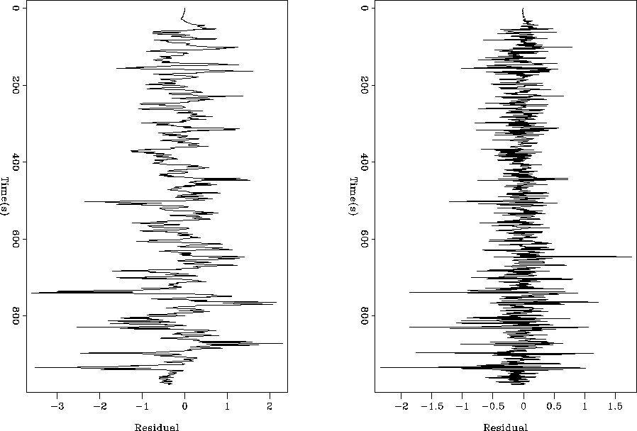
Now we have almost all of the pieces to create multiple realistic interval velocity models from our $\bf v_{rms}$ measurements. The left panel of Figure  shows the residual after estimating the model using (15). We can see that there is a low frequency component to the residual. We can estimate a PEF from this residual and resolve (15) using

$$\bf N= \bf H \bf V \bf D_1,$$ (16)

where $\bf H$ is convolution with our PEF calculated from the residual. The resulting residual (right panel of Figure ) is now white.

 

dix3 Figure 14 The left panel is the residual without using a whitening filter. The right panel is the residual using a whitening filter. Note how the residual is showing only minimal structure.

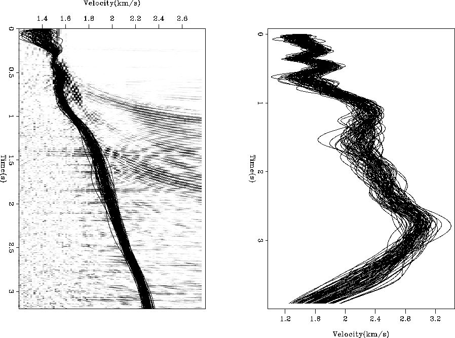
We can now use our multiple realization machinery to produce multiple interval velocity models that have approximately the correct covariance. The right panel of Figure  shows 80 interval velocity realizations. The left panel shows those realizations converted back to $\bf v_{rms}$. Note how the $\bf v_{rms}$ functions stay within variance bounds. In addition, as we expected, we see larger variance where our bounds are wider. 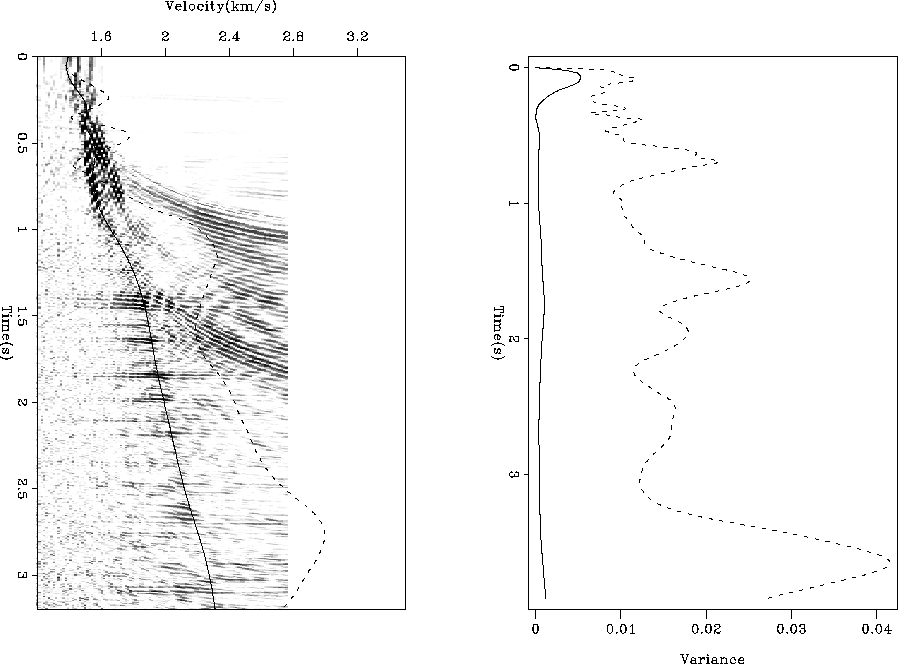If we look at the mean and variance of our interval and rms (Figure ) estimates we get another interesting result. Areas of large variance are not always correlated.

 

dix4
Figure 15 The right panel shows 80 interval velocity realizations. The left panel show those interval velocities converted back to $\bf v_{rms}$ overlaying the stack power for the CMP gather.

 

dix5 Figure 16 The left panel shows the mean of the $\bf v_{rms}$ (solid line) and $\bf v_{int}$ (dashed line) of 80 realizations overlaying the stack power. The right panel shows the variance of $\bf v_{rms}$ and $\bf v_{int}$ for the 80 realizations.