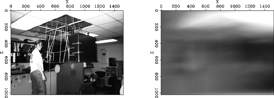
![[*]](http://sepwww.stanford.edu/latex2html/cross_ref_motif.gif) shows the model
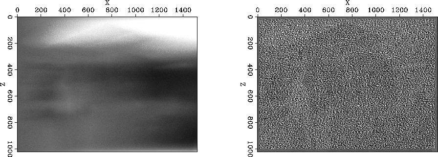
shows the model ![[*]](http://sepwww.stanford.edu/latex2html/cross_ref_motif.gif) shows the data
shows the data ![[*]](http://sepwww.stanford.edu/latex2html/cross_ref_motif.gif) ),
we can quickly get an unreasonable model estimate (right
panel of Figure
),
we can quickly get an unreasonable model estimate (right
panel of Figure ![[*]](http://sepwww.stanford.edu/latex2html/cross_ref_motif.gif) ).
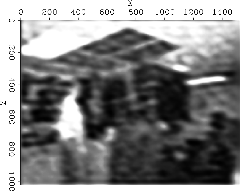
If we add an isotropic regularizer, our estimate
improves substantially (Figure
).
If we add an isotropic regularizer, our estimate
improves substantially (Figure ![[*]](http://sepwww.stanford.edu/latex2html/cross_ref_motif.gif) ).
We will speed up the
conversion of our problem
by preconditioning the problem
).
We will speed up the
conversion of our problem
by preconditioning the problem | |
||
| (10) |
 |
![[*]](http://sepwww.stanford.edu/latex2html/movie.gif)
 |
![[*]](http://sepwww.stanford.edu/latex2html/movie.gif)
|
rand2
Figure 5 The model estimated from the data shown in the left panel of Figure ![[*]](http://sepwww.stanford.edu/latex2html/cross_ref_motif.gif) using an isotropic regularization operator. using an isotropic regularization operator.
|  |