IID Residuals

A more difficult, but at times more realistic, challenge is when our noise is not Gaussian. The left panel of Figure  shows smoothed Gaussian noise, of approximately the same amplitude as the random noise used above, that we will add to our data (right panel of Figure ). The resulting model estimate (right panel of Figure ) shows a clear imprint of the noise pattern. If we look at the $\bf r_{d}$ vector (left panel of Figure ), we see that we have disobeyed both of the IID requirements. The residual is definitely correlated and if we look at histogram of the residuals (right panel of Figure ), the identically distributed requirement looks suspect.

 

iid
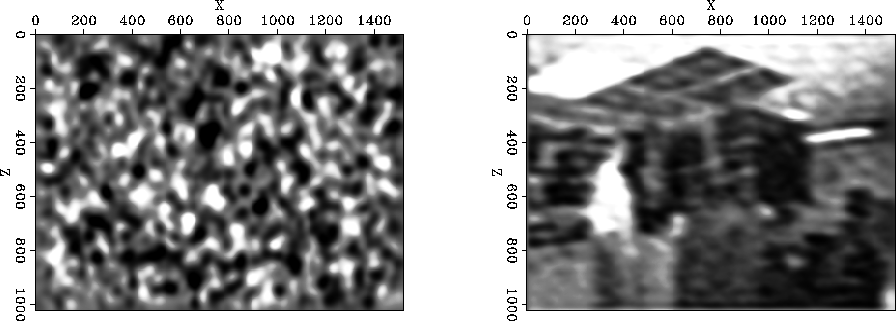
Figure 6 The left panel shows correlated noise that we are going to add to our data. The right panel shows the resulting inversion. Note how the imprint of the noise is visible in the model.

 

iid2
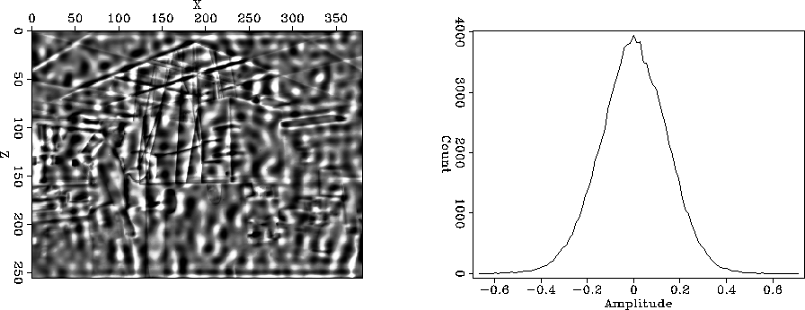
Figure 7 The left panel shows the residual ($\bf r_{d}$)associated with the model in Figure . The right panel is a histogram of the residual. Note the structure in the residual and the deviation from Gaussian of the residual.

Up to this point we have ignored the inverse noise covariance matrix $\bf N$. Claerbout (1999) and Guitton (2000) suggested using a PEF for $\bf N$ estimated from the residual. If we do this we get an improved result (left panel of Figure ) and a more decorrellate residual (right panel of Figure ). Remember that $\bf N$ should be the inverse of the noise spectrum. Estimating it from the residual does not necessarily give us the same information. Since this is a synthetic example, we have another option. We can estimate $\bf N$ directly from our noise estimate. Figure  shows the result of the inversion using this filter and the $\bf r_{d}$ vector associated with the inversion. The resulting estimate is generally of higher quality.

 

iid3
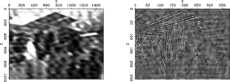
Figure 8 The left panel shows the inversion result using a PEF estimated from the residual as $\bf N$.The right panel shows the resulting $\bf r_{d}$. Note the improved result compared to Figure .

 

iid4
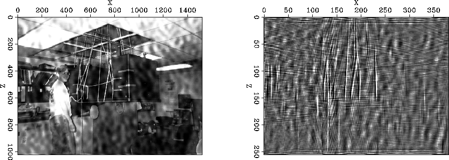
Figure 9 The left panel shows the inversion result using a PEF estimated from the known noise as $\bf N$.The right panel shows the resulting $\bf r_{d}$. Note the improved result compared to Figure . Compared to Figure  we see an improvement in image clarity at some expense of a boosting of the noise.