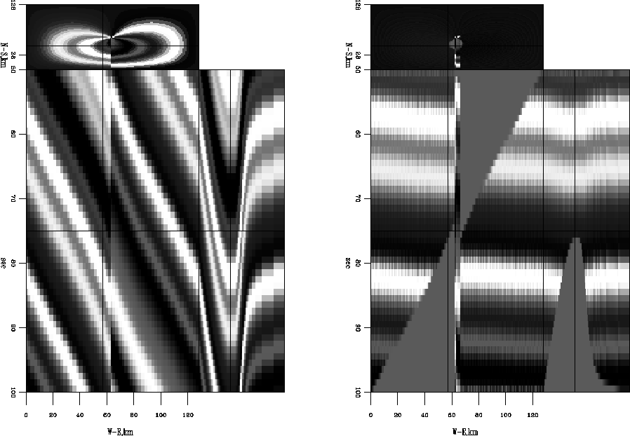Faulted model - test case

 

parking.2D_sm
Figure 1 Faulted model. Left is unflattened. Right is flattened. It does a poor job because it calculates erroneous dips at the fault.

 

parking.time
Figure 2 Same as Figure except solved in T-X space rather than Fourier. This allows a weight to be applied to remove fitting equations corrupted by bad dips at the fault. Notice it does a much better job at flattening.

 

parking_3D.time
Figure 3 Faulted model in T-X using 3-D integration

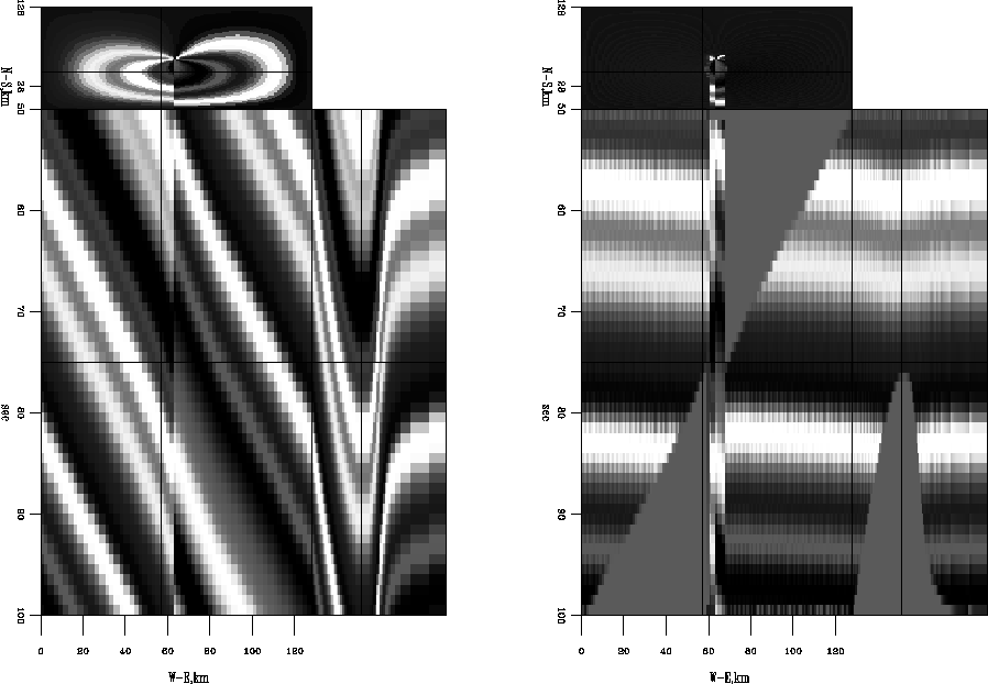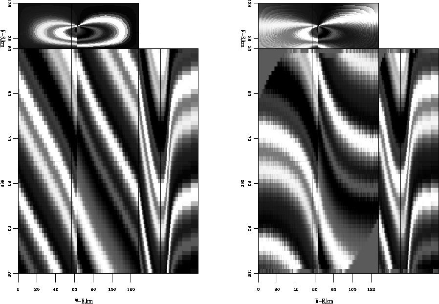
The synthetic model seen in Figure has a fault starting from the center. The dip is constant with depth. Surfaces within this model gradually climb in the clockwise direction, much like a parking garage. This model is flattened using a Fourier space method in Figure . Because of erroneous dips at the fault, it does a poor job of flattening. Figure shows the results of applying the T-X space approach using conjugate gradients and a weight that throws out fitting equations at the fault as in equation (10). Notice it is now well flattened. Similarly, using the 3-D integration version in T-X space, shown in Figure , the results are adequately flattened.

Although completely separated fault blocks present an obvious challenge to this method because the dip is unknown at fault discontinuities, I have some plausible solutions. The fault slip displacement would be the perfect dip information at a fault. If you have a fault block that is bounded on all sides by faults within the 3-D cube, then there is really no way to remove the deformation across the faults without at least knowing two points that correlate on each side of the fault. From an interpretation standpoint it will be necessary to restore both sides of the fault to see the best geological picture. Under such circumstances it maybe necessary to first calculate the fault contours of the fault using a method similar to that described in Lomask (2002) and put the values of the fault slip into the dip cube as input into the flattening process. This fault contour procedure basically just cross-correlates both sides of each fault.

The weights applied to the residual, equation (9), to throw out fitting equations at faults and to weaken fitting equations with low dip semblance or high noise can be created from rough fault models or coherency cubes. Additionally, this method still can be integrated with automatic fault tracking schemes. The output from these programs can be passed to my flattening scheme and used as fault weights. The fault contours, which are an easy output from the flattening method, can be used to quality check and improve the automatic fault tracking output.