


Next: Inversion of the Hessian
Up: Least-squares solution of the
Previous: Least-squares solution of the
Let us define the  block matrix M as follows:
| 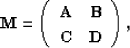 |
(87) |
where A, B, C, and D are matrices.
First, we consider the matrix equation
| 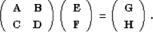 |
(88) |
If we multiply the top row by  and add it to the bottom,
we have
and add it to the bottom,
we have
|  |
(89) |
Then we can easily find F and E. The quantity  is called the Schur complement of A and,
denoted as
is called the Schur complement of A and,
denoted as  , appears often in linear algebra Demmel (1997).
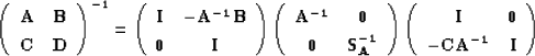
The derivation of F and E can be written in a matrix form
, appears often in linear algebra Demmel (1997).
The derivation of F and E can be written in a matrix form
| 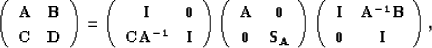 |
(90) |
which resembles an LDU decomposition of M.
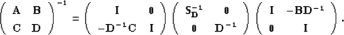
Alternatively, we have the UDL decomposition
| 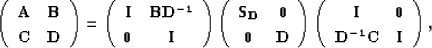 |
(91) |
where 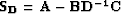 is the Schur complement of
D.
The inversion formulas are then easy to derive as follows:
is the Schur complement of
D.
The inversion formulas are then easy to derive as follows:
|  |
(92) |
and
|  |
(93) |
The decomposition of the matrix M offers opportunities for
fast inversion algorithms. The final expressions for M are
| 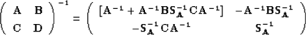 |
(94) |
and
| ![\begin{displaymath}
\left( \begin{array}
{cc}
{\bf A} & {\bf B} \\ {\bf C} & ...
...[{\bf D^{-1}}+{\bf
D^{-1}CS_D^{-1}BD^{-1}}]\end{array}\right).\end{displaymath}](img281.gif) |
(95) |
Equations (![[*]](http://sepwww.stanford.edu/latex2html/cross_ref_motif.gif) ) and () yield the matrix inversion lemma
) and () yield the matrix inversion lemma
|  |
(96) |
Next: Inversion of the Hessian
Up: Least-squares solution of the
Previous: Least-squares solution of the
Stanford Exploration Project
5/5/2005