Reverse Time Migration of up and down going signal for ocean bottom data

The RTM operator

Since there are many different ways to implement reverse time migration, we must specify how we construct our RTM operator. Our model space is the reflectivity of the subsurface. It is computed by cross-correlating the source wavefield with the receiver wavefield injected backward in time,

$$m(\bold x) = \sum_{\bold s} \sum_{t} u_s (\bold x, t, \bold s) u_r (\bold x, t, \bold s) ,$$ (3)

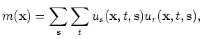where $\bold s$ marks the location of the source, $t$ is the time, $\bold x$ represents a point in the sub-surface, $m(\bold x)$ is the reflectivity of the sub-surface, and $u_s (\bold x, t, \bold s)$ and $u_r(\bold x, t, \bold s)$ are the source and receiver wavefields at location $\bold x$, time $t$, and shot location $\bold s$. Our reverse time migration is set up so that $u_s (\bold x, t, \bold s)$ and $u_r(\bold x, t, \bold s)$ are computed using a background velocity model, $V_o (\bold x)$ and the constant-density acoustic wave equation:

$$\frac{1}{V_o^2} \frac{d^2 u}{d t^2} = \nabla^2 u .$$ (4)

In our finite differencing scheme, we approximate the Laplacian to fourth order in space and the time derivative to second order in time. Note that in this study, we only migrate with the correct velocity. The correct velocity is smoothed to avoid spurious cross-correlation artifacts.

For ocean-bottom data, the receiver ghost reflection is very valuable, because when applied with mirror imaging, it produces better sub-surface illumination than the primary event. This claim will be apparent from later results. To create overlapping of the receiver ghost for ocean bottom RTM, we must have a reflecting top boundary.

Reverse Time Migration of up and down going signal for ocean bottom data