Results on the data

I use the shot-gather wz27 (Western Geophysical, Alaska), which is described and displayed on Figure 1. The ocean floor being hard, the water-bottom multiples and peglegs are strong, and you can notice them on Figure 1; the lag at 0-offset is approximately 120 ms.

 

H27input
Figure 1 Shot-gather wz27. (a) Time-offset section: dt=$4\ msec$, dx=$50\ m$.(b) $\tau-p$ domain: p=0., dp=$0.02\ s.km^{-1}$. In both cases, strong peglegs multiples can be seen, with a lag approximately equal to 120 msec.

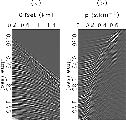
The figure 1 also displays the $\tau-p$ transform of this shot-gather. The strong events at $p=0.7 \ s.km^{-1}$ are due to the presence of strong direct arrivals, and head-waves. The water-bottom peg-legs are still very easy to recognize. Notice also that the event at 1.5 seconds is stronger than the previous events. Actually, it seems that the primaries are stronger with time; this property justifies the use of adaptive algorithms.

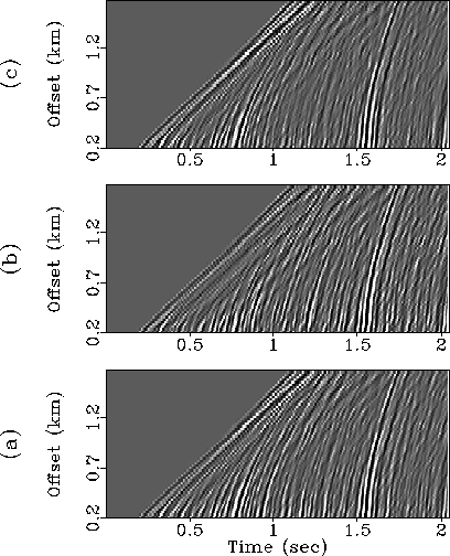
To see the effects of this process, I apply three algorithms, with the same length for the filter (n=30). The first one consists of a block method: I solve the minimization problem on time windows of 800 msec (200 samples), with a classical Levinson algorithm; the windows overlap by half their length. The second is the LSL algorithm, with no tapering ($\lambda=1$). It is interesting to observe what happens before the event at 1.5 sec, because the LSL residuals before this event are supposed not to be influenced by it. The third algorithm is the general Burg's adaptive filtering, with $\lambda=0.97$, and no windowing. Each of these algorithms is applied on each trace separately.

I display the results on Figure 2, with which we can compare the outputs of the three processes with the input in the $\tau-p$ domain on Figure 1.

 

H27topdemul
Figure 2 Removal processing in the $\tau-p$ domain. (a) Block method. (b) LSL algorithm. (c) Adaptive Burg-type algorithm. The peglegs are better attenuated by the LSL and Burg-type methods than by the block algorithm. However, a new undetermined event (1.2 sec) appears after LSL processing; it is not present on the output of the Burg-type algorithm.

The Burg-type algorithm seems more robust that the LSL algorithm. The different multiples are efficiently suppressed. Effectively, the Burg-type algorithm takes into account the events after 1.5 sec: they provide a lot of information on the multiplication process, because they are stronger than the previous events. On the other hand, up to this time (1.5 sec), the LSL algorithm does not take them into account, so that the process is less stable. Notice also a better lateral continuity on the residuals of the Burg-type algorithm. This suggests a better numerical stability of this algorithm, less sensitive to incoherent noise.

 

H27result
Figure 3 Removal processing, output in the time-offset domain. (a) Block method. (b) LSL algorithm. (c) Adaptive Burg-type algorithm. The outputs of Figure 2 are transformed back to the time-offset domain. The Burg-type method is more efficient in the elimination process. In particular, after velocity analysis, the undetermined event at 1.2 sec on (b) appeared to be a water-bottom pegleg of the primary at 0.7 sec.

A doubt could still persist about the undetermined event at 1.2 sec on the residuals of the LSL algorithm. However, I transformed back the residuals in the $\tau-p$ domain to the time-offset domain, as shown on Figure 3. After applying a velocity analysis on the LSL residuals, it appeared that this event was a pegleg multiple of another primary at 0.7sec. Was it an artifact of the process, or a real unpredictable multiple? I don't know indeed, but it confirms the instability of this algorithm.