


Next: EXAMPLES
Up: ADDING ANISOTROPY
Previous: Theory
The isotropic F(u)
in Van Trier and Symes is  in cartesian coordinates
and
in cartesian coordinates
and  in polar ones.
For our examples we shall restrict ourselves to transverse isotropy
with a vertical axis of symmetry, one of the simplest types of anisotropy.
in polar ones.
For our examples we shall restrict ourselves to transverse isotropy
with a vertical axis of symmetry, one of the simplest types of anisotropy.
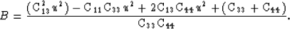
F(u) in this case for ``simple'' cartesian coordinates is
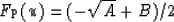
for qP waves and
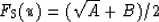
for qS waves, where
| 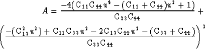 |
(5) |
| |
and
In principle, there is no theoretical obstacle to extrapolation in
polar coordinates,
but in that case F(u) becomes much worse than
equation (5). For that reason, we have remained
with the simpler cartesian extrapolation method for our preliminary
examples here. (Of course we could have followed Vidale's lead
and used expanding square calculation fronts. However, this would
have put ``corners'' of the calculation fronts right where we wanted
to model shear triplications. We decided to stick with simple extrapolation
in z for now, so we know the strange wavefront shapes are from the
anisotropy, not the finite-difference method.)
Again, in principle, there should be no objection to using the upwind
finite-difference method that worked so well in Van Trier and Symes.
In practice the upwind method has proven surprisingly recalcitrant.
One possible reason is that the quantity  required by the
upwind method (it is defined by
required by the
upwind method (it is defined by  )is typically quite complicated, both in behavior and to calculate.
(In the isotropic case it is ridiculously easy:
)is typically quite complicated, both in behavior and to calculate.
(In the isotropic case it is ridiculously easy:  .)
.)
For the examples in this paper we use the two-step Lax-Wendroff method.
This is a fixed-stencil second-order method (Press et al., 1988).
Theoretically this second-order method should be more accurate
than the first-order upwind method, but it is difficult to predict
the behavior of various finite-difference methods in practice.
Symes suggests that any fixed-stencil method
should be unstable for this application (Symes, 1990).
Next: EXAMPLES
Up: ADDING ANISOTROPY
Previous: Theory
Stanford Exploration Project
1/13/1998