


To perform residual-velocity analysis, we need to find RMO equations that describe how the image of a reflector moves as a function of the offset between the surface locations of the reflector and the shot. By substituting relation (10) and equation (7) into (8), we have
 |
(11) |
![]()
This pair of parametric equations defines the RMO equation
for a common depth point
(xt, zt) where the dipping angle of the reflector is ![]() .As we mentioned before,
if the migration velocities are not equal to the actual
velocities of the media, the image of the reflector moves away both
horizontally and vertically from the
actual position of the reflector. Therefore
the residual-moveout curve for the CDP is three-dimensional.
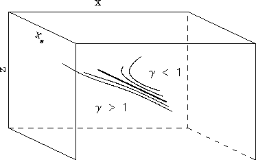
Figure 4 shows the residual moveout curves for a given
reflector location (xt, zt), with dipping angle
.As we mentioned before,
if the migration velocities are not equal to the actual
velocities of the media, the image of the reflector moves away both
horizontally and vertically from the
actual position of the reflector. Therefore
the residual-moveout curve for the CDP is three-dimensional.
Figure 4 shows the residual moveout curves for a given
reflector location (xt, zt), with dipping angle ![]() and velocity ratio
and velocity ratio
![]() .
.
 |

 |
The application of equation (11) requires the random access of whole
3-D dataset. This process is usually expensive and perhaps unnecessary for
mildly varying structures. Let us assume that the structures are so smooth
that, within the range of horizontal movement of the image
(due to velocity errors), the
lateral variation of the dipping angle of the reflector
can be neglected. Under this assumption,
we can consider the RMO in common-surface-location
gathers. In Appendix B, we show that for a given surface location x, depth
zt, dipping angle ![]() and velocity ratio
and velocity ratio ![]() , the RMO equation
for a CSL is
, the RMO equation
for a CSL is
 |
(12) |