1-D inversion

In this section, we will apply the previous technique to the inversion of traveltimes for a cross-well geometry. Synthetic data were generated through the 1-D isotropic model shown in Figure , using a geometry of 17 sources and 17 receivers equally spaced at the source and receiver well respectively. If we plot the components of the slowness vector $\mbox{\boldmath$S$}$(equation(4)) for this model, we obtain the profile shown at the right hand side of Figure . Both slowness components are identical because the model is isotropic. In this example, the slowness contrast between the background and the anomalous layer is small ($1 \%$) and therefore, the propagation of the energy can be safely modeled by straight ray paths.

 

syn-model
Figure 3 Synthetic isotropic model used to test the algorithm. At the right, it is shown the slowness vector S that describes this model.

 

1d-synthetic Figure 4 Result of the inversion of the synthetic data generated through the model shown in Figure 3.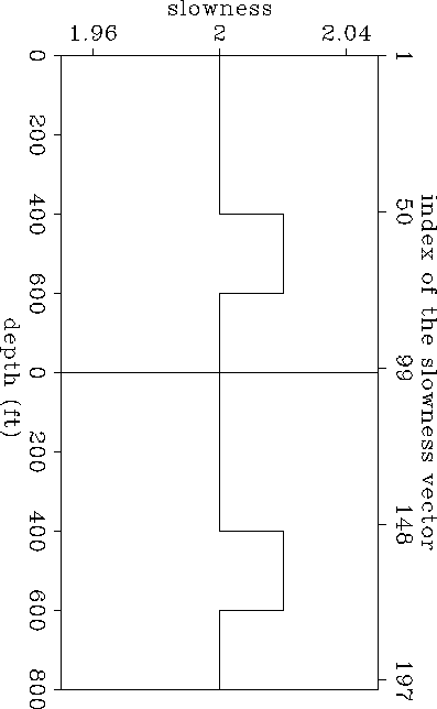

We can constrain the inversion by allowing only vertical variations in the model if it is know a priori that the medium is layered. Doing this we eliminate instabilities and non-uniqueness in the inversion associated with lateral variations, remaining only those associated with the vertical component of the slowness, which is not sampled propperly by the recording geometry.

The image area was divided into 100 layers of equal thickness (8 ft). The inversion process has to estimate 200 parameters from 289 traveltimes. Figure  shows the slowness vector obtained after 60 conjugate gradients (CG) iterations. There is no difference between the given S (Figure ) and the estimated one (Figure ). Note also that the results can be represented as a function of depth as well as a function of the index of the slowness vector. In the two next results the depth axis will be omitted.

Figure  shows the convergence toward the result as a function of the CG-iterations. The result shown in Figure  correspond in Figure  to 60 CG-iterations in the axis number of iterations. The two ``hills'' represent the slowness at the anomalous layer. We say that convergence has been achieved when the top and the bottom of the hills are flat. Note that the horizontal component of the slowness converges faster than the vertical component. This is because in the given model, the horizontal component of the slowness in the anomalous layer is better sampled than the vertical component: the range of ray angles (absolute values) is from to 53 degrees ($53 \approx \arctan (\frac{800}{600})$)which is a typical range for cross-well experiments.

 

cg-600x800
Figure 5 Variations of the slowness vector as a function of the number of conjugate gradient iterations. The original model is shown at the top.

If the same geometry is used to generate synthetic data through the model shown at the top of Figure  (were the well to well separation has been decreased), we obtain that both components converge at the same rate. This is because the vertical component of the slowness is better sampled than before: the range of ray angles varies between and 76 degrees ($76 \approx \arctan (\frac{800}{200})$).

 

cg-200x800
Figure 6 Variations of the slowness vector as a function of the number of conjugate gradient iterations. The only difference between the model shown at the top and the model of Figure 3 is in the horizontal dimension.

The previous results tell us that if it is not possible to perform ``enough'' iterations in order to reach the flat top of both hills ( Figures  and ), we may wrongly conclude that the medium is anisotropic. What is really happening is that the components of the slowness vector do not converge at the same rate. Severe limited view problems as well as low signal to noise ratio are some reasons that may limit the amount of CG-iterations that can be performed before the ill-conditioning of the problem starts playing any role.