

Next: USING PREDICTION TO DESIGN
Up: WEIGHTED LEAST-SQUARES
Previous: Linear scheme
The first few iterations of the CG algorithm lower the
energy in the regions where the semblance of the original data was high,
but the remaining problem is that the subsequent iterations still
focus to much attention in the same places because the weighting
function stays the same. To overcome this restriction we need a variable
weighting operator that is reevaluated after a given number of steps of the
CG solver, resulting in the reformulation of equation (4)
as an iterative linearization of a nonlinear problem. Each external step i
of the CG solver will work on the residuals  defined as
|  |
(5) |
where

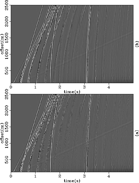
Figure ![[*]](http://sepwww.stanford.edu/latex2html/cross_ref_motif.gif) show the results of the linear and nonlinear
semblance weighting schemes. Although with less artifacts in the shallow
reflections, and with less deterioration in the primaries (notably the
near offset of the primary at 1.6 seconds) relative to the
non-weighted algorithm, they fail to eliminate the set of
reverberations in the shallow part of the gather.
Furthermore, at the near offset traces the multiples are not
suppressed, as is usually the case in velocity-domain-based methods.
show the results of the linear and nonlinear
semblance weighting schemes. Although with less artifacts in the shallow
reflections, and with less deterioration in the primaries (notably the
near offset of the primary at 1.6 seconds) relative to the
non-weighted algorithm, they fail to eliminate the set of
reverberations in the shallow part of the gather.
Furthermore, at the near offset traces the multiples are not
suppressed, as is usually the case in velocity-domain-based methods.
multw01
Figure 3 Results of (a) the multiple suppression using the linear pre-weighted
scheme described by equation (4) and (b) multiple
suppression using the nonlinear preweighted scheme described by
equation (5). In both cases the synthetic dataset of
Figure ![[*]](http://sepwww.stanford.edu/latex2html/cross_ref_motif.gif) is used as input.
is used as input.


Next: USING PREDICTION TO DESIGN
Up: WEIGHTED LEAST-SQUARES
Previous: Linear scheme
Stanford Exploration Project
12/18/1997
![]()
![[*]](http://sepwww.stanford.edu/latex2html/cross_ref_motif.gif) show the results of the linear and nonlinear
semblance weighting schemes. Although with less artifacts in the shallow
reflections, and with less deterioration in the primaries (notably the
near offset of the primary at 1.6 seconds) relative to the
non-weighted algorithm, they fail to eliminate the set of
reverberations in the shallow part of the gather.
Furthermore, at the near offset traces the multiples are not
suppressed, as is usually the case in velocity-domain-based methods.
show the results of the linear and nonlinear
semblance weighting schemes. Although with less artifacts in the shallow
reflections, and with less deterioration in the primaries (notably the
near offset of the primary at 1.6 seconds) relative to the
non-weighted algorithm, they fail to eliminate the set of
reverberations in the shallow part of the gather.
Furthermore, at the near offset traces the multiples are not
suppressed, as is usually the case in velocity-domain-based methods.

![[*]](http://sepwww.stanford.edu/latex2html/cross_ref_motif.gif) is used as input.
is used as input.