REVIEW OF CLAERBOUT'S RECURSIVE DIP FILTER

The recursive dip filter, invented by Claerbout (1985), works in the time and space domain. It is more attractive for seismic data processing than a dip filter that operates in the frequency-wavenumber domain, because it can be temporally and spatially nonstationary. In addition to time and space variability, the recursive dip filter offers the advantage of a simple and economic recursive implementation.

Let P denote raw data and Q denote filtered data in the frequency-wavenumber domain. Dip filtering can be achieved by using a low-dip-pass filter:

$$Q(\omega, k) = {\alpha \over{\alpha+({k^2\over -i\omega})}}P(\omega, k),$$ (1)

or a high-dip-pass filter:

$$Q(\omega, k) = {({k^2\over -i\omega})\over{\alpha+({k^2\over -i\omega})}}P(\omega, k),$$ (2)

where $\omega$ is the temporal frequency, k is the spatial frequency, and $\alpha$ determines the cutoff dip (Claerbout, 1985).

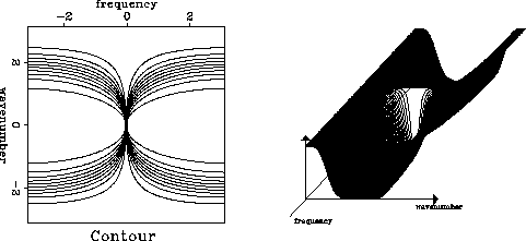
To understand the recursive dip filter, we need to examine its amplitude spectrum. Figure 1 shows the amplitude spectrum of a high-dip-pass filter. The spectrum changes slowly from a pass zone to a reject zone. This is the only drawback of recursive filters, however, the transition zone need not be short in our application to trace interpolation.

 

fig1
Figure 1 Left: contour plot of the amplitude spectrum of a high-pass recursive dip filter with $\alpha = 0.5$ Right: 3D plot of the amplitude spectrum of the same filter.

The realization of equations (1) and (2) is obtained by replacing $-i\omega$ and -k² with $\partial \over \partial t$ and $\partial^2 \over \partial x^2$, respectively. Clearing out all the fractions in equation (1) then leads t the following partial-differential equation:

$$\alpha({\partial q \over \partial t} - {\partial p \over \partial t}) = \alpha{\partial^2 q \over \partial x^2}.$$ (3)

Approximating the derivative by a difference operator gives the desired recursive relations (Claerbout, 1985). For example, the low-pass filter becomes

$$({\alpha\over \Delta t} + {1\over 2 \Delta x^2}T)q_{t+1} = (... ...over 2 \Delta x^2}T)q_t + {\alpha\over \Delta t}(p_{t+1}-p_t) ,$$ (4)

where T represents a tridiagonal matrix with ( 1, -2, 1 ) along the diagonal, and $\alpha$ determines the cutoff dip. For a stable and accurate implementation, we apply the Crank-Nicholson method and the 1/6 trick. The result is the following differencing star:

$$(-1-\beta)q_t^{x-1}+p_t^{x-1} (-{1\over b}+2+2\beta)q_t^x+({1\over b}-2)p_t^x (-1-\beta)q_t^{x+1}+p_t^{x+1}$$

$$(1-\beta)q_{t+1}^{x-1}-p_{t+1}^{x-1} ({1\over b}-2+2\beta)q_{t+1}^x+({1\over b}-2)p_{t+1}^x (1-\beta)q_{t+1}^{x+1}-p_{t+1}^{x+1}$$

where $\beta = {\Delta t \over 2\alpha b \Delta x^2}$ and $b = {1 \over 6}.$

Implementation of the above differencing star is straightforward. However, in order to develop the forward and transpose operators needed for iterative application, we need to write these operators in a matrix form as shown in the following section.