RESULTS

Interpolation of missing traces is carried out iteratively using a conjugate-gradient algorithm, which minimizes the high-dip-pass-filtered output of NMO-corrected CMP gathers. Finally, inverse NMO processing is applied with the same velocity as was used in the NMO correction. To preserve the amplitude of the original data, we use pseudounitary NMO processing (Claerbout, 1991).

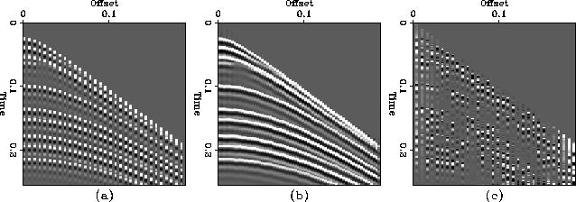
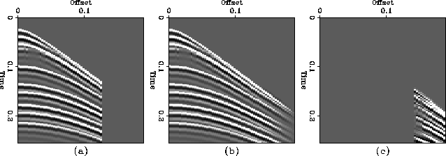
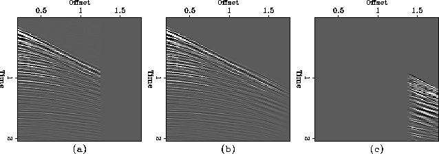
In order to test the validity of the proposed method, it has been applied to several sets of synthetic and real data. Figure 4 shows a synthetic CMP gather with interlaced missing traces, the result of interpolation, and the difference between the original traces and the interpolated traces. Similarly, Figure 5 shows a synthetic CMP gather with truncation at the end, the result of interpolation, and the difference between the original traces and the interpolated traces. 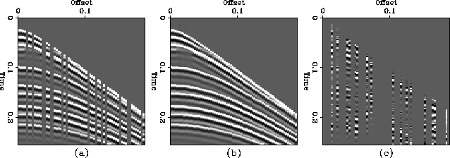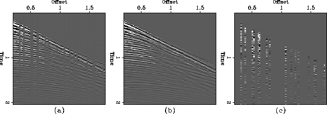In Figure 6 a synthetic CMP gather with random missing traces is shown, along with the result of interpolation and the difference between the original traces and the interpolated traces.

 

fig4
Figure 4 (a) Synthetic CMP gather with interlaced missing traces, (b) the result of interpolation, and (c) the difference between original and interpolated traces.

 

fig5
Figure 5 (a) Synthetic CMP gather with truncation at the end, (b) the result of interpolation, and (c) the difference between original and interpolated traces.

 

fig6
Figure 6 (a) Synthetic CMP gather with randomly missing traces, (b) the result of interpolation, and (c) the difference between original and interpolated traces.

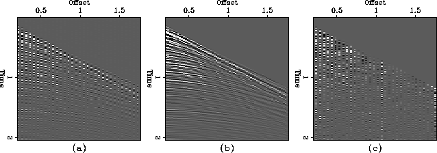
Figures 7, 8 and 9 show the processing of a real dataset. The data set, wz27 (Yilmaz and Cumro, 1983), has been windowed to provide a small test dataset. Normal moveout was applied to the data using water velocity, making most events reasonably, but not perfectly, flat. Figure 7 shows the results of interpolating the dataset when odd-number traces were zapped to produce missing traces. The difference between the original traces and interpolated traces is also shown. Figure 8 shows the result of the interpolation and the interpolation error for a truncated CMP gather. Figure 9 shows the result of interpolation for random missing traces.

 

fig7
Figure 7 (a) Real CMP gather with interlaced missing traces, (b) the result of interpolation, and (c) the difference between original and interpolated traces.

 

fig8
Figure 8 (a) Real CMP gather with truncation at the end, (b) the result of interpolation, and (c) the difference between original and interpolated traces.

 

fig9
Figure 9 (a) Real CMP gather with randomly missing traces, (b) the result of interpolation, and (c) the difference between original and interpolated traces.

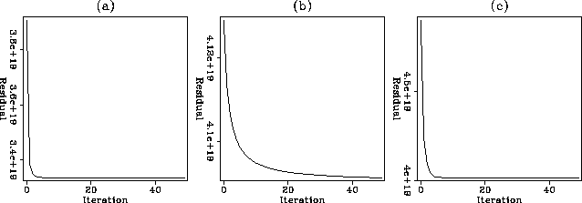
Figure 10 shows residuals as a function of the iteration number for the three missing trace types. We see that all cases converge very fast, and that interlaced and random missing traces converge in just a few steps.

 

fig10
Figure 10 Residuals with respect to iteration for (a) interlaced missing traces, (b) truncation at the end, and (c) randomly missing traces.