Constant velocity

The first example is a constant velocity model of 2.0 km/s and dimensions of 6 km on a side. The first known source position is at ${\bf x}_1$ = 0.0 km, and the second known source position is at ${\bf x}_3$ = 6.0 km, which represents a very sparse traveltime table spatial separation of 6 km. (Of course, for constant velocity and v(z) models, the traveltimes depend only on offset and depth, and are independent of lateral source position. In this regard, the comment on sparse sampling is relevant only in terms of interpolation, and is not relevant to what I would actually do in practice!) Their respective traveltime fields $\tau_1$ and $\tau_3$ are plotted in Figure . The horizontal and vertical traveltime gradient fields at ${\bf x}_1$ are denoted as $\tau_{1x}$ and $\tau_{1z}$ respectively, and are plotted in Figure . The horizontal and vertical traveltime gradient fields at ${\bf x}_2$ are denoted as $\tau_{3x}$ and $\tau_{3z}$ respectively, and are plotted in Figure .

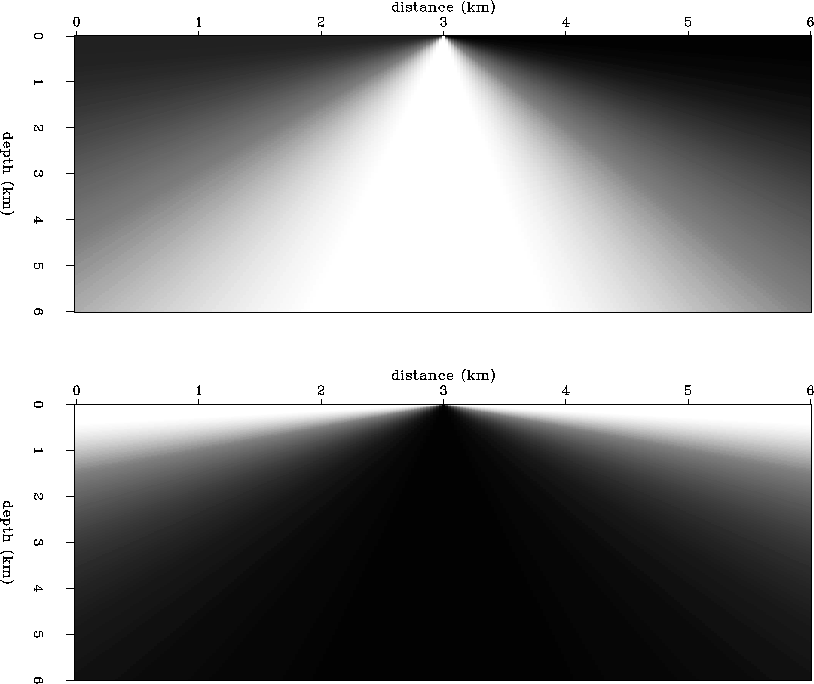
The interpolated traveltime field $\tau_2({\bf x};{\bf x}_2)$ at ${\bf x}_2$ = 3.0 km is plotted in the top panel of Figure , and the traveltime gradients $\tau_{2x}$ and $\tau_{2z}$ are plotted in Figure . The relative interpolation traveltime error is contoured in the lower panel of Figure . The contour farthest from the desired source position at 3.0 km has a value of 1%, and increases to 10% relative error as you move in toward the source position, in 1% contour value increments. In theory, this example should be error-free since the $\cos\theta$ terms are given exactly by (8) in a constant velocity medium. For this example, the interpolated traveltimes are accurate to within 1% relative error, my rule of thumb requirement, over most of the subsurface space, using a sparse shot interval of 6 km. However, there is evidence of some small numerical inaccuracy and a resulting tendency of singularity right at the source position, where the $\theta$ values change rapidly and are therefore most sensitive to error. Hence, in more general velocity models, we should expect instability near the source region.

 

c13t
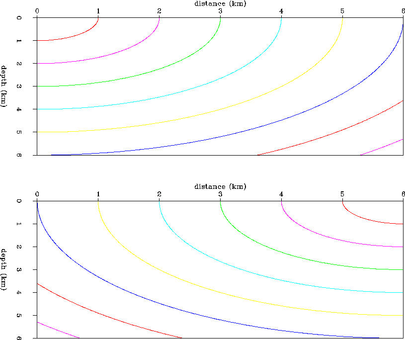
Figure 2 Constant velocity model. Contours of traveltime field for the two given surface source positions at 0.0 km (top) and 6.0 km (bottom).

 

c1xz
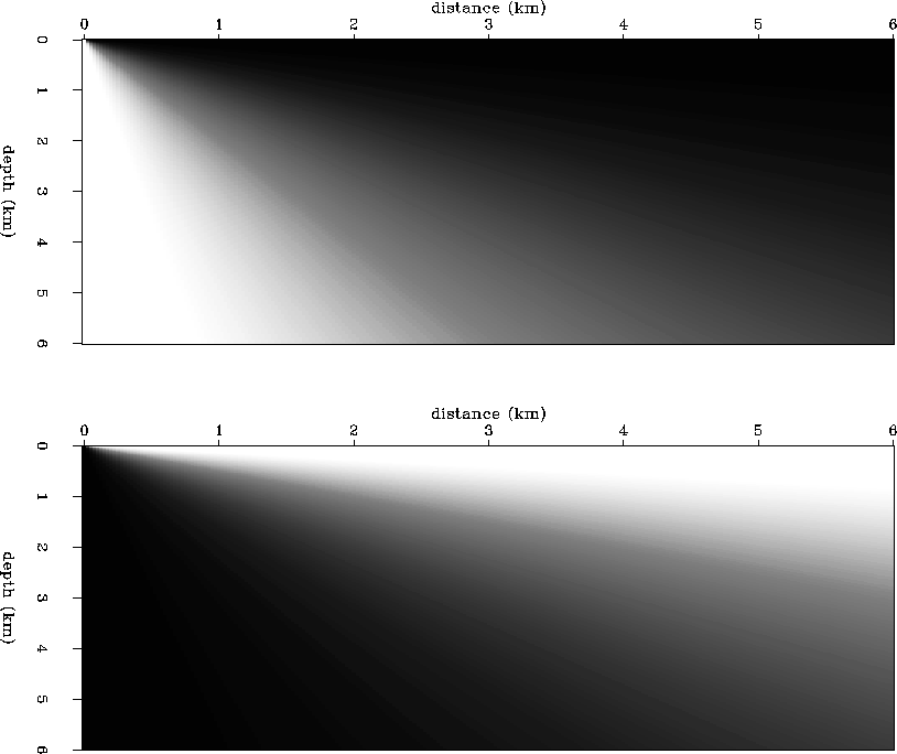
Figure 3 Constant velocity model. Horizontal (top) and vertical (bottom) traveltime gradient fields for the surface source positioned at 0.0 km.

 

c3xz
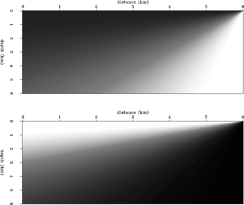
Figure 4 Constant velocity model. Horizontal (top) and vertical (bottom) traveltime gradient fields for the surface source positioned at 6.0 km.

 

cite
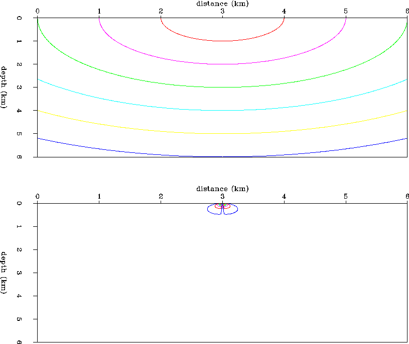
Figure 5 Constant velocity model. Interpolated traveltime field. The top panel is the interpolated traveltime field for a surface source positioned at 3.0 km. The lower panel is the relative error between the interpolated traveltime field, and the correct traveltimes modeled by an analytical solution to the eikonal. The contour farthest from the source region is at 1% relative error, and the contour values increase to 10% error right at the source location, in 1% contour increments.

 

cixz
Figure 6 Constant velocity model. Horizontal (top) and vertical (bottom) traveltime gradient fields for the interpolated surface source positioned at 3.00 km.