References

• Byun, B. S., Corrigan, D., and Gaiser, J. E., 1989, Anisotropic velocity analysis for lithology discrimination: Geophysics, 54, 1564-1574.

• Dellinger, J., and Muir. F., 1988, Imaging reflections in elliptically anisotropic media: Geophysics, 53, 1616-1618.

• Dellinger, J., 1991, Anisotropic seismic wave propagation: Ph.D. thesis, Stanford University, Stanford, California, USA.

• Garmany, J., 1989, A student's garden of anisotropy: Ann. Rev. Earth Planet. Sci., 17, 285-308.

• Gonzalez, A., Lynn, W., and Robinson, W.F. IV, 1991, Prestack Frequency-Wavenumber (f-k) Migration in a Transversely Isotropic Medium: Expanded Abstracts of the 61st Annual International Meeting of the SEG, 1155-1157.

• Jones, E. A., and Wang, H. F., 1981, Ultrasonic velocities in Cretaceous shales from the Williston basin: Geophysics, 46, 288-297.

• Knuth, D. E., 1981, The art of computer programming, volume 2: seminumerical algorithms: Addison-Wesley, Reading, Massachussetts, USA.

• Schoenberg, M., and Muir, F., 1989, A calculus for finely layered anisotropic media: Geophysics, 54, 581-589.

• Sena, A. G., 1991, Seismic traveltime equations for azimuthally anisotropic and isotropic media: Estimation of interval elastic properties: Geophysics, 56, 2090-2101.

• Wolfram, S., 1988, Mathematica: A System for Doing Mathematics by Computer: Addison-Wesley, Reading, Massachussetts, USA.

 

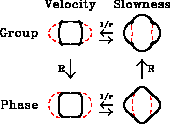
Group-four
Figure 1 Plots of group velocity (impulse response), group slowness, phase velocity, and phase slowness (dispersion relation) for the qSV mode of Greenhorn Shale (thick solid line) and the elliptically anisotropic vertical-paraxial approximation (thin dashed line). The four plots are connected by only two transformations, here labeled ``1/r'' and ``R''. The transformation ``1/r'' (invert the radial coordinate) is its own inverse, as is the combined transformation ``$R \circ {1/r}$'' that goes from group velocity to phase slowness (and vice versa). The combined transformation also maps ellipses onto ellipses. (Garmany, 1989) and (Dellinger, 1991)  

 

Sample
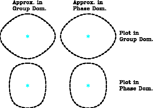
Figure 2 The curves that result for three different values of the F factor in equation (10); the asterisks mark the origin. On the left, F = 3/7; in the middle F = 1 and the curve is an ellipse; on the right F = 7/3.  

 

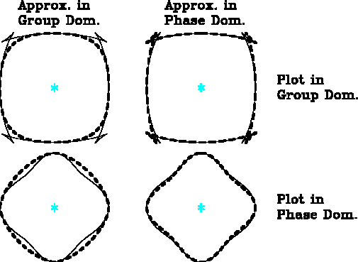
Compare.s.1
Figure 3 Group-velocity and phase-slowness plots of the qP surface of Greenhorn shale (thin solid line) and the corresponding first anelliptic approximation (thick dashed line). On the left the approximation is made in the group-velocity domain; on the right the approximation is made in the phase-slowness domain. The approximations are consistent to within about two percent.  

 

Compare.s.-1
Figure 4 As in Figure 3, but for the considerably more anisotropic qSV surface. The approximations in the two domains are not consistent around the triplication.  

 

perfect
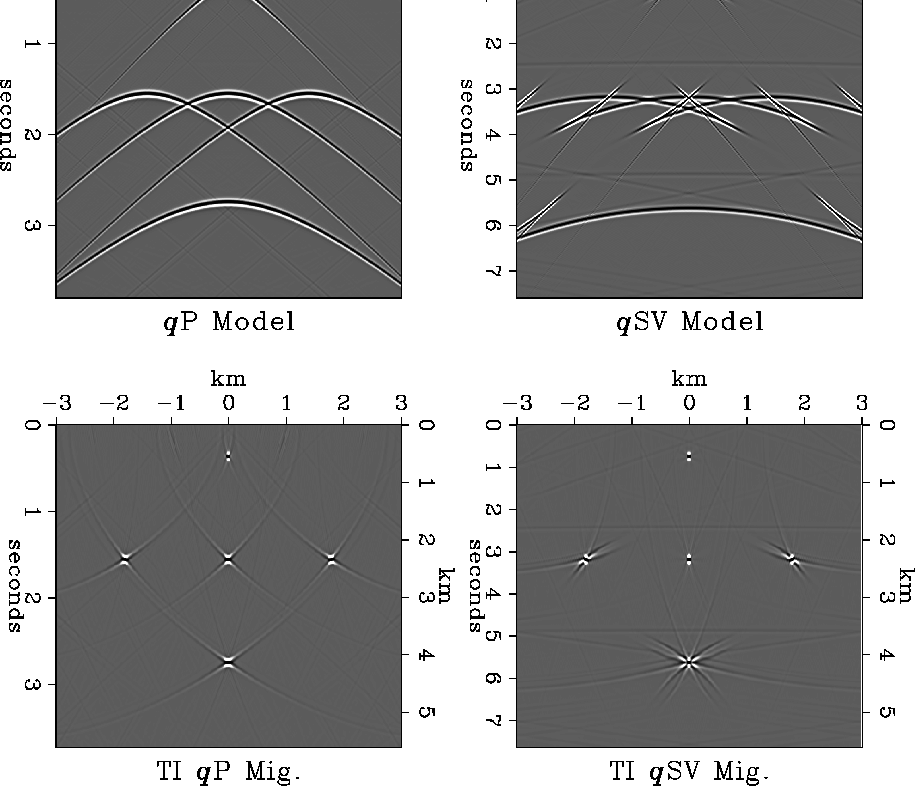
Figure 5 Scalar Stolt modeling and migration for qP and qSV waves in a TI medium. (W₁₁=13.72, W₁₃=4.28, W₃₃=9.08, W₄₄=2.16, and W₆₆=4.24, all in km/s.) Top: qP and qSV models resulting from four point reflectors arranged in a diamond-shaped lattice. Bottom: Exact Stolt migrations of the modeled data. The hyperboloids do not completely collapse back to points because of the truncations at the model edges.  

 

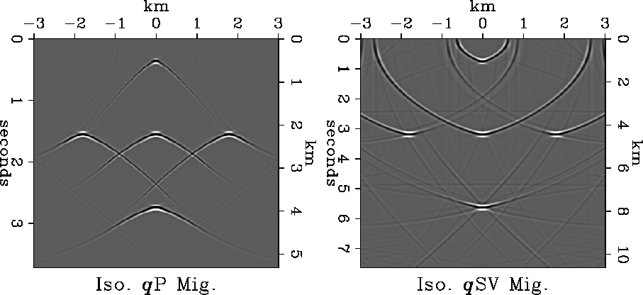
approxI
Figure 6 Approximate isotropic migrations of the exact TI models in Figure 5. The P migration velocity (left) was $V_{{\mbox{\rm\protect\scriptsize P}},x{\mbox{\rm\protect\scriptsize NMO}}}=2.8554$ km/s; the S migration velocity (right) was $V_{{\mbox{\rm\protect\scriptsize SV}},x{\mbox{\rm\protect\scriptsize NMO}}}=2.780$ km/s.  

 

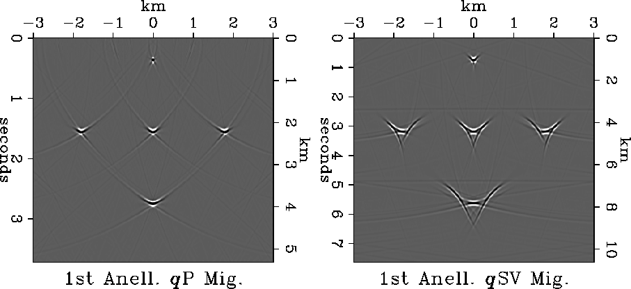
approxA1
Figure 7 Approximate migrations of the exact TI models in Figure 5 using the first anelliptic approximation. For the qP waves, the migration used $V_{{\mbox{\rm\protect\scriptsize P}},z} \equiv V_{{\mbox{\rm\protect\scriptsize P}},x{\mbox{\rm\protect\scriptsize NMO}}} =2.8554 km/s$,and $V_{{\mbox{\rm\protect\scriptsize P}},x}=3.7041$ km/s. For the qSV waves, the migration used $V_{{\mbox{\rm\protect\scriptsize SV}},z} \equiv V_{{\mbox{\rm\protect\scriptsize SV}},x{\mbox{\rm\protect\scriptsize NMO}}} =2.7797$ km/s, and $V_{{\mbox{\rm\protect\scriptsize SV}},x}=1.4697$ km/s. (The unconstrained vertical velocities are set equal to the moveout velocities to conform to the usual practice; the vertical scale thus chosen has no effect on the time migration.)  

 

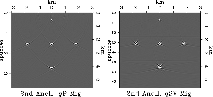
approxA2
Figure 8 Approximate migrations of the exact TI models in Figure 5 using the second anelliptic approximation. For the qP waves, the migration used $V_{{\mbox{\rm\protect\scriptsize P}},x{\mbox{\rm\protect\scriptsize NMO}}}=2.8554$ km/s, $V_{{\mbox{\rm\protect\scriptsize P}},z}=3.0133$ km/s, $V_{{\mbox{\rm\protect\scriptsize P}},x}=3.7041$ km/s, and $V_{{\mbox{\rm\protect\scriptsize P}},z{\mbox{\rm\protect\scriptsize NMO}}}=2.3974$ km/s. For the qSV waves, the migration used $V_{{\mbox{\rm\protect\scriptsize SV}},x{\mbox{\rm\protect\scriptsize NMO}}}=2.7797$ km/s, $V_{{\mbox{\rm\protect\scriptsize SV}},z}\equiv V_{{\mbox{\rm\protect\scriptsize SV}},x}=1.4697$ km/s (from the symmetry of TI), and $V_{{\mbox{\rm\protect\scriptsize SV}},z{\mbox{\rm\protect\scriptsize NMO}}}=2.3436$ km/s. In this migration the vertical scale is assumed to be known.  

 

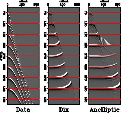
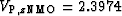
NMOfig
Figure 9 Anelliptic moveout removal. The model consists of 8 layers and a halfspace, the top layer 75 time-units thick and all others 50 time-units thick. The layer moveout velocities from top to bottom are .25, .3, .4, .45, .3, .3, .45, and .5. (Units are arbitrary.) All layers but the one from time 175 to 225 are isotropic. The single anisotropic layer, fourth down, corresponds to the qSV mode for elastic parameters W₁₁=.81, W₁₃=.3645, W₃₃=.8505, and W₅₅=.243. (The qSV moveout velocity is .45.)