


Cross-well data were recorded at the McElroy field, a carbonate reservoir of the Permian Basin in west Texas. This field has large oil reserves. It was discovered in 1926 and has been under continuous water-flooding since the early 1960s. McElroy field produces mainly from intertidal and shallow-shelf dolostones and siltstones of the Grayburg formation, which is a stratigraphic/structural trap. Hydraulic fracturing has stimulated reservoir performance. Porosity and permeability data from cores show that the Grayburg formation is very heterogeneous, with significant changes over short distances. The reason for the heterogeneity is that anhydrite and gypsum have plugged the pores (Avasthi et al., 1991). Structurally, the region is flat with mildly increasing dips at the bottom of the surveyed section (Lazaratos et al., 1992). The profile area is part of three 20-acre, five-spot patterns in a CO2 pilot study.
A cylindrical
piezoelectric bender was used as the source, a linear upsweep from
250 to 2000 Hz.
Well spacing is 184 feet.
The receiver well in the cross-well profiling
was an observation well drilled for the CO2 study, and
the receiver
system was a nine-level array of hydrophones.
The plane of the survey is almost perpendicular to the
direction of natural fractures measured in a nearby well
(Avasthi et al., 1991).
The target of the experiment was a reservoir between 1850 and 1960 feet.
Sources and receivers were centered around the
reservoir, from 1650 to 2150
feet.
[Reservoir depths are changed
for purposes of presentation in this paper.]
The vertical spacing between sources and receivers was 2.5 feet.
The survey
consists of nearly 36 000 traces (201 sources ![]() 178 receivers)
sampled at 0.2 ms.
More details about the data acquisition can be found in Harris et al. (1992).
178 receivers)
sampled at 0.2 ms.
More details about the data acquisition can be found in Harris et al. (1992).
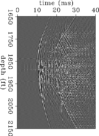
Figure ![[*]](http://sepwww.stanford.edu/latex2html/cross_ref_motif.gif) shows a common receiver gather recorded at 1880 feet.
Data editing and geometry definition was performed before picking the
data.
The total number of traveltimes
picked from the field data
was 33 519 and 20 887 for P-waves and S-waves, respectively.
Van Schaack et al. (1992)
show that the source can be modeled as a radial horizontal point
source, which
explains why
no shear waves are clearly visible in the
data for ray angles less than
shows a common receiver gather recorded at 1880 feet.
Data editing and geometry definition was performed before picking the
data.
The total number of traveltimes
picked from the field data
was 33 519 and 20 887 for P-waves and S-waves, respectively.
Van Schaack et al. (1992)
show that the source can be modeled as a radial horizontal point
source, which
explains why
no shear waves are clearly visible in the
data for ray angles less than ![]() degrees with respect to the horizontal, as Figure shows.
degrees with respect to the horizontal, as Figure shows.
 |

P-wave energy is converted to shear energy at the source well. If the source well is perfectly cylindrical, and if the downhole source is positioned symmetrically within the source well, the polarization of the converted energy recorded at the receiver well is contained in the plane of the survey. Therefore, it is safe to assume that most of the recorded shear energy in this experiment corresponds to the SV-mode.
The P-wave traveltimes used for the inversion were from sources and receivers forming angles between 9 and 36 degrees with the horizontal. Even though the corresponding range of ray angles may be slightly different depending on how strong the velocity contrasts are, I still expect most ray angles at all layers to fall within the range of validity of the elliptical approximation. By applying this constraint on the data aperture, the number of P-wave traveltimes was reduced to 12 258 from the original 33 519. For similar reasons, the number of S-wave traveltimes was reduced to 2922, which corresponds to sources and receivers forming angles between 29 and 35 degrees.
The initial model
for the tomographic inversion of P-wave traveltimes
is homogeneous isotropic. The model is described by 200 horizontal
layers of equal thickness
(2.5 feet). Figure shows
the elliptical velocities that result after inverting the data.
![]() is larger than VP,x in some
strata, which indicates that
the anisotropy is not caused by fine, horizontal layering.
The mean absolute value of the residuals
for this model
is 0.086 ms.
is larger than VP,x in some
strata, which indicates that
the anisotropy is not caused by fine, horizontal layering.
The mean absolute value of the residuals
for this model
is 0.086 ms.
|
mcroy-p
Figure 9 P-wave elliptical velocities estimated from field data. Thick line: VP,x. Thin line: | 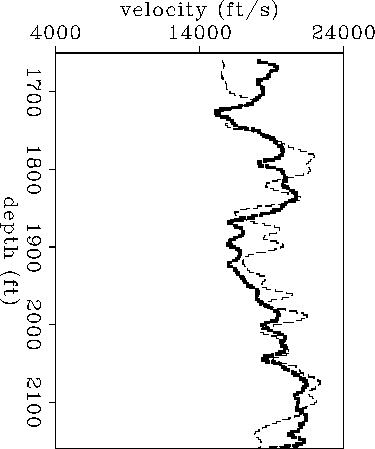 |
Figure shows
the elliptical velocities that result from the inversion of
shear-wave traveltimes. The initial model in this case was also
homogeneous isotropic and described by 200 layers of equal thickness.
Seven layers were eliminated during the inversion procedure.
![]() is close to
is close to ![]() ,which means that, as discussed also in section 2.7,
the P-wave
anisotropy at this site is close to elliptical.
As Figures and show,
the shear-wave anisotropy at this site is smaller than
the compressional wave anisotropy.
The mean absolute value of the residuals computed for the model
in Figure is 0.240 ms, approximately equal to the
sampling interval.
,which means that, as discussed also in section 2.7,
the P-wave
anisotropy at this site is close to elliptical.
As Figures and show,
the shear-wave anisotropy at this site is smaller than
the compressional wave anisotropy.
The mean absolute value of the residuals computed for the model
in Figure is 0.240 ms, approximately equal to the
sampling interval.
|
mcroy-s
Figure 10 S-wave elliptical velocities estimated from field data. Thick line: | 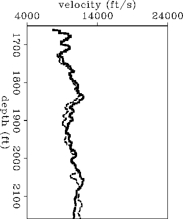 |
Finally, the elliptical velocities of Figures
and are transformed into elastic constants
at each depth. Figure
shows the result of the transformation.
V11 and V33 (horizontal and vertical
P-wave velocities, respectively) vary more rapidly than
V44 (SV-wave velocity).
V33
is almost the same as ![]() because the shear
wave anisotropy is not significant, as Figure shows.
The difference V11 - V33
alternates between zero or negative
in the interval between 1700 and 2100 feet.
If we assume that the
anisotropy is caused by fine layering,
such changes in V11 - V33 can be explained
by a sequence of isotropic and anisotropic strata with horizontal
axes of symmetry, probably vertically fractured.
The reservoir between 1850 and 1960 feet corresponds to one
stratum that is probably vertically fractured, which suggests
that other intervals where V11 < V33 may also correspond
to vertically-fractured reservoir zones.
because the shear
wave anisotropy is not significant, as Figure shows.
The difference V11 - V33
alternates between zero or negative
in the interval between 1700 and 2100 feet.
If we assume that the
anisotropy is caused by fine layering,
such changes in V11 - V33 can be explained
by a sequence of isotropic and anisotropic strata with horizontal
axes of symmetry, probably vertically fractured.
The reservoir between 1850 and 1960 feet corresponds to one
stratum that is probably vertically fractured, which suggests
that other intervals where V11 < V33 may also correspond
to vertically-fractured reservoir zones.
|
mcroy-elastic
Figure 11 Elastic constants at the McElroy site (in units of velocity) estimated from the elliptical velocities of Figures 9 and 10, assuming a TI medium. Dotted line: V44. Thick-dashed line: V13. Dotted-dashed line: V11. Thin-dashed line: V33. | 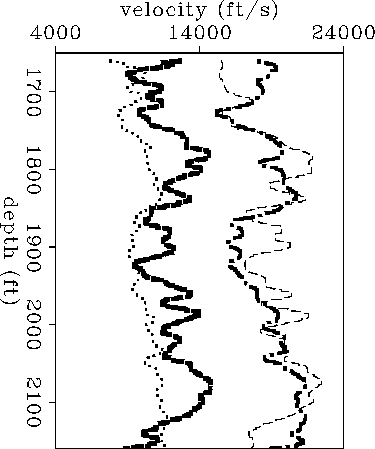 |
Figure compares the horizontal and
vertical velocities estimated from the cross-well measurements
with the vertical shear and compressional velocities derived
from the sonic log. Comparing
shear-wave velocities yields the results expected
for a TI medium:
the vertical
shear velocity from the sonic log is the same as the
horizontal shear velocity derived from cross-well measurements.
For the compressional velocities, however, the results are not
as expected: the sonic log velocity is closer to
the horizontal velocity than to the vertical velocity
estimated from
cross-well traveltimes.
|
mcroy-elastic-logs
Figure 12 Elastic constants (in units of velocity) estimated from cross-well traveltimes compared with sonic logs blocked every six feet. Continuous line at the left: shear sonic velocity. Continuous line at the right: compressional sonic velocity. Dotted line: V44. Dotted-dashed line: V11. Thin-dashed line: V33. | 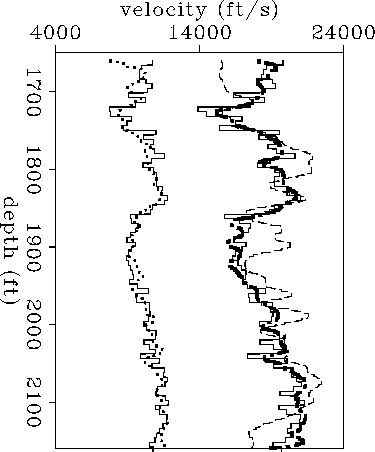 |
The differences between vertical P-wave sonic velocity and vertical P-wave velocity estimated from cross-well traveltimes can be explained in several ways that are consistent with the idea of vertically fractured strata alternating with isotropic strata. One explanation is that fluids used when drilling can penetrate the reservoir zones causing a decrease in the compressional velocities of waves that travel close to the well without affecting either the velocities of waves that travel far from the well or the shear velocities. Another explanation assumes that the vertical fractures are embedded in a slow, fluid-filled matrix. The fractures are well-separated and filled with fast material (anhydrite), which can effectively increase the vertical velocity of waves that travel vertically in the interwell region without affecting either the velocity of waves that travel horizontally (because the fractures are thin) or the velocity of high-frequency waves that travel around the borehole in the low-velocity matrix. Strong, lateral heterogeneities in the vertical component of the velocity may cause the type of variation observed in the results, because the model doesn't account for them. This possibility, however, is less likely because reflection images of the site show fairly laterally homogeneous layers (Lazaratos et al, 1992).
Having out-of-plane shear arrivals would help to confirm the hypothesis of vertical fractures, by allowing us to look at the shear-wave splitting in the near horizontal direction.