INTRODUCTION

Kjartansson 1979 showed that shallow absorption or velocity anomalies can masquerade as gas-bearing bright spots. (For a brief summary see 1985.)  Kjartansson showed that the bright-spots masquerade is easily uncovered by making a plot of energy in some time gate as a function of midpoint and offset. His plot shows streaking generally aligned with the shot axis and with the geophone axis whereas an amplitude streak resulting from a small bright spot should be aligned on a constant midpoint. More careful examination shows that the alignments of Kjartansson's data are not precisely along the shot and geophone axes, but they are tilted slightly towards the midpoint axis. For my recalculation of Kjartansson's figure, see Figure 1.

 

kjamp
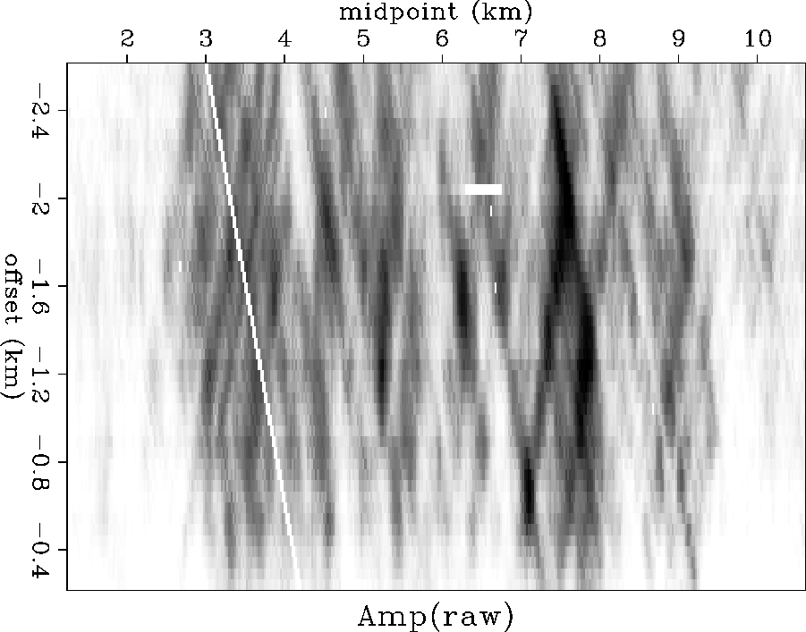
Figure 1 Kjartansson's Grand Isle data, root-mean-square energy in the time interval 2.0-2.6 sec, after NMO with velocity 2.05.

Kjartansson interprets the tilt as a measure of depth of burial of the anomaly and he slant stacks to provide a map of anomaly depth versus midpoint. (Actually he does better than slant stack, he attempts a planar decomposition). In Figure 1 there is a pronounced streak at a $45^\circ$ angle associated with a missing shot. A missing shot is equivalent to perfect absorption directly under the shot, so this $45^\circ$ streak corresponds to zero depth under the shot. Likewise, if we were to see a $45^\circ$ streak of opposite orientation, it would correspond to zero depth under the geophone. A vertical streak corresponds to absorption at the reflector under the midpoint. At any depth, there are two applicable angles, one tipping one way (for shots) and one tipping the other (for geophones).

Kjartansson does not analyze anomalies with regard to whether they result from absorption or focusing, but those of us who have worked with migration for many years tend to regard all amplitude variations as focusing phenomena because focusing so easily gives amplitude variations. Kjartansson shows one NMO corrected CMP gather that clearly shows time shifts, but when he assembles a plane of times in midpoint-offset space, alignments of interesting events are not so clear as with amplitudes. His slant stack of this plane is disappointing compared to his amplitudes. (Those seismologists who believe that observational seismology gives reliable timing measurements but unreliable amplitude measurements will be surprised by Kjartansson's very convincing results.) In summary, Kjartansson's work showed clearly the locations of likely lateral-velocity variation anomalies, but provided no direct path toward building a best fitting velocity model.

A variety of factors led me to revisit this data and its analysis: Two members of our group had developed wave-equation datuming code and were about to struggle with the problem of estimating the velocity model. Computers are much more powerful than they were when Kjartansson did his work. Kjartansson's data (or a subset) were recently found and loaded on our machines. My recent research direction, data adaptive multidimensional filters (DAMF), encouraged me to believe that I could readily accomplish potentially complicated corrections, prediction of one shot profile from another, for example, without need for an elaborate theory. I suspected that DAMF might provide the missing components needed to create a near surface (top 500 ms) lateral velocity variation model using only its distortion of deep reflections and so I set out to try.

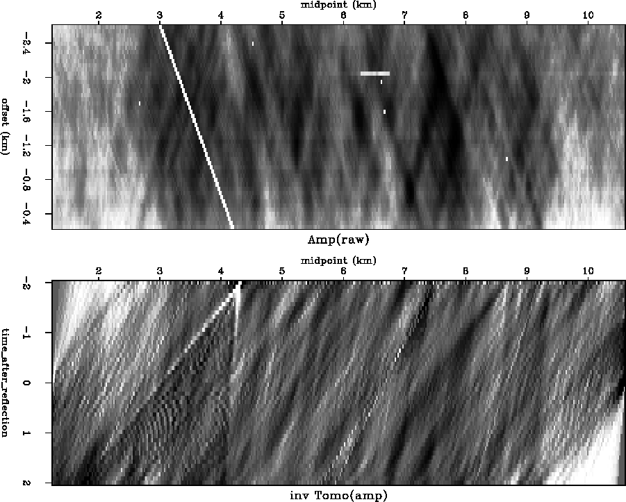
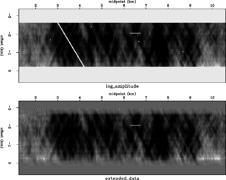
Figures 2-4 show various slant-stack like transformations of the logarithm of the amplitude in Figure 1.

 

kartom.0
Figure 2 Top shows the log amplitude of the energy in a time gate from 2.0-2.6s (after NMO with v=2.05). Bottom shows a slant stack ranging from common shot to common geophone. Think of the vertical axis on the bottom plot as ranging along the ray path. The missing shot streak on the top panel becomes a clipped impulse function on the bottom at km=4.2 and time=-1.0. The missing shot streak truncates at near offset and at far offset. The near-offset truncation gives a near vertical streak through the clipped impulse. The wide-offset truncation gives a near $45^\circ$ streak through the pulse. Geophysically interesting are about a dozen ``blobs'' on the bottom frame about 300-600ms from the earth surface either on the shot path or geophone path.

 

extend
Figure 3 Top is the logarithm of amplitude as in Figure 2 except that it is padded. Bottom shows the padded amplitude after extension from an initial guess that the logarithm take on its mean value. Failure to fill in a short line segment from about 6 to 7km at about 2km offset results from the mask program assuming that only zero-valued data is missing. The extension uses a prediction filter predicting in the upward direction, so the upward side shows stronger short wavelengths than the downward side.

 

kartom.2
Figure 4 Repetition of Figure 2 with extended data.

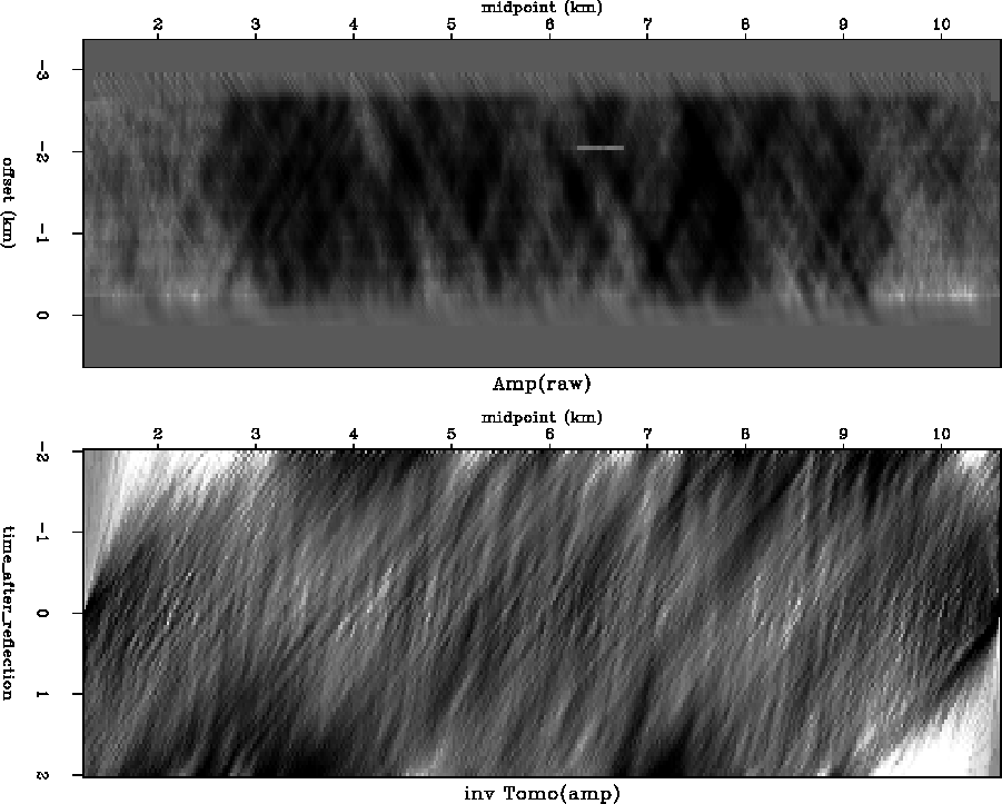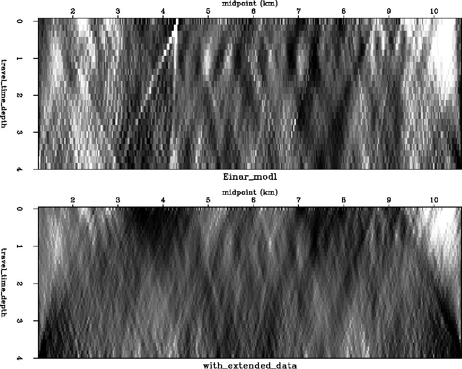
To mimic Kjartansson's plot of amplitude versus midpoint and depth, I folded and summed the bottoms panels of each of Figure 2 and Figure 4 about t=0 thereby combining information from the upgoing and downgoing path. The result is shown in Figure 5.

 

einarmodl
Figure 5 Tomographic distribution of energy with midpoint and traveltime depth. Top is for amplitudes before extension, bottom is after.