INTERPOLATION AND LEAST SQUARES

The basis of the interpolation scheme is very simple. Data, which may be irregular, poorly sampled, have missing offsets, etc. are transformed to coordinates of zero-offset time and velocity. This velocity spectrum is then used to model data at the desired offsets.

This may be formulated simply, but not effectively, as follows Ji (1994). Estimation of the velocity spectrum for a given CMP gather is done by solving the equation

d = Hm

where d is the recorded data, m the model in velocity space, and H the forward operator which creates a hyperbola in the data space from a spike in the model space. Interpolating in this manner does not yield satisfying results. The reason is in the null space of the operator H.

Solving this problem by conjugate gradients yields a model which predicts the recorded data very well. However, even for perfect hyperbolas, the final model will not be exact. Spikes will tend to be smoothed, and some noise is inevitable. This difference does not impact the model's ability to predict the data because, as Nichols 1994 points out, the difference between the exact model and the inversion result is in the null space of the operator. However, changing the data space, which me must do in order to interpolate or regularize, changes the null space. Thus, the slight artifacts in the velocity space, which model nothing in the original data space and thus do not contribute to the residual (which resides in the original data space), will model nonzero energy into a different data space, creating artifacts.

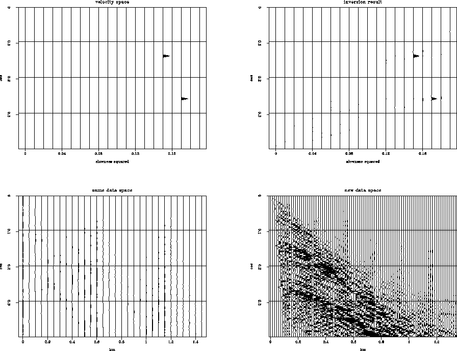
Figure 1 shows a simple example of a null space changing as data space changes. On the top left of Figure 1 is a velocity space with two spikes in it. The top right is the velocity space estimated by inversion. The bottom left is the difference between the two top panels used to model into the same data space as was used in the inversion. The bottom right is again modeling using the difference between the top two panels, but this time into a new, finely-sampled data space. Note that much more energy has appeared in the new data space. The max values in the bottom right panel are 100 times those in the bottom left panel. The null space of the operator has changed. The large amplitudes in the bottom right are about one third the amplitude of the spikes in the model space (top left of the figure), and of the hyperbola amplitudes in data space. This should represent an unacceptable interpolation artifact.

 

null-space
Figure 1 Null space effects: Top left and right are original and estimated velocity spaces. Bottom left is difference between top figures modeled into original data space. Bottom right is difference between top figures modeled into different data space.