INVERSION OF SYNTHETIC DATA: EFFECT OF LAYERING

In this section we examine the effect of layering on the inversion results. Assuming that the near seafloor sediments are underlain by a hard layer will result in interference effects between the signals from the seafloor and the one from the interface between the first and second layer. Using a hard layer simulates the extreme case of subsurface structure effects, and will thus produce upper error bounds for the inverted ocean-bottom parameters. We explore the effects for a layer which is either 100 m or 50 m thick. The synthetics were generated using the same parameters as described in the previous section. The acoustic/elastic properties of the water and the two layers are shown in Table 4.

$$\rho_2$$ layer v_p2 (m/s) v_s2 (m/s)

water 1500 - 1050

1 1693 437 1900

2 2141 781 2100

Table 4: Properties of the water and the two layers underlying the water.

 

layer100 Figure 10 Vertical particle motion for a 100 m thick layer.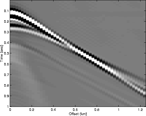

 

vxl100 Figure 11 Radial particle motion for a 100 m thick layer.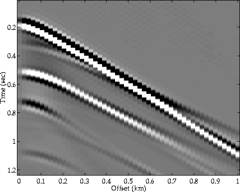

 

pl Figure 12 Pressure for a 100 m thick layer.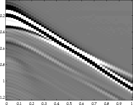

Figures 10, 11, and 12 show the synthetic seismograms for the vertical particle velocity, radial particle velocity and the pressure for the near sea-bottom layer being 100 m thick. In the case of a 50 m thick layer, the interference of the signals will appear at smaller offsets.

Prior to the inversion of the data for the near seafloor parameters, the arrivals of the wave that is being reflected off the second layer were muted out, leaving only the signals generated by the seafloor (Figures 13, 14, 15). Those signals were then transformed into the ($\omega - k$) domain, in which the reflection and AVO coefficients were determined.

 

vzl Figure 13 Vertical particle motion for a 100 m thick layer after muting.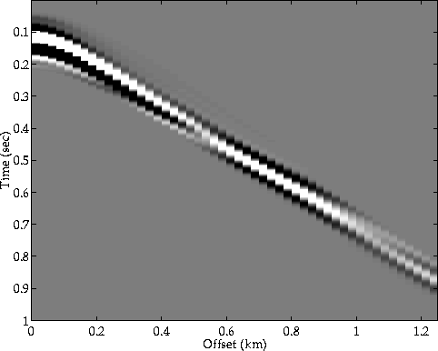

 

vxl100m Figure 14 Radial particle velocity for a 100 m thick layer after muting.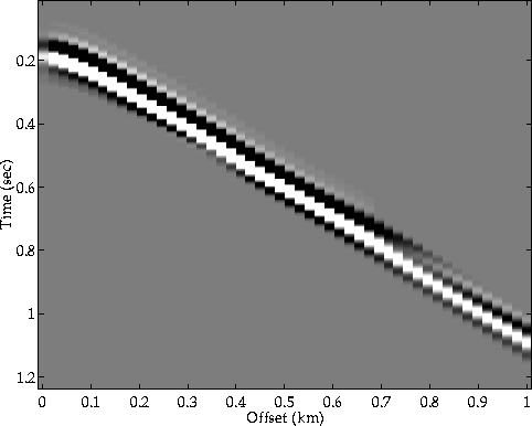

 

plm Figure 15 Pressure for a 100 m thick layer after muting.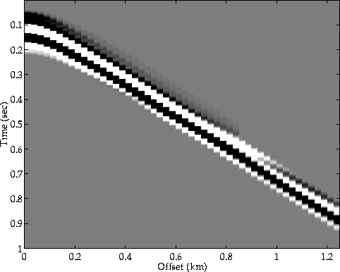