 |
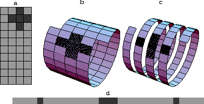
Figure 6 Filtering on a helix. The same filter coefficients overlay the same data values if the 2-D coils are unwound into 1-D strips.
Computational work on a 2-D Cartesian mesh sometimes requires a Fourier transform on one of the axes. A byproduct is that the original plane becomes a cylinder--no real problem when the diameter of the cylinder is large enough. The helix idea involves a similar compromise. Take the Cartesian mesh to be a collection of columns. Instead of connecting the bottom of each column to its top getting a cylinder, the helix connects the bottom of one column to the top of the next. The columns all connect into a supercolumn, a one-dimensional space. The mesh can be parameterized either as a 1-D space or as a 2-D space. The first surprising thing is what the helix does to convolutions and partial differential equations.
A basic idea of filtering, be it in one dimension, two dimensions, or more, is that you have some filter coefficients (finite-differencing star) and some sampled data; you pass the filter over the data; at each location you find an output by crossmultiplying the filter coefficients times the underlying data and then summing the terms. Figure 6 shows a helical mesh for 2-D data on a cylinder.
 |
Darkened squares depict a 2-D filter shaped like the Laplacian operator. The input data, the filter, and the output data are all on helical meshes all of which could be unrolled into linear strips. A compact 2-D filter like a Laplacian, on a helix is a sparse 1-D filter having long empty gaps.
Since the values output from filtering can be computed in any order, we can slide the filter coil over the data coil in any direction. The order that you produce the outputs is irrelevant. You could compute the results in parallel. We could, however, slide the filter over the data in the screwing order that a nut passes over a bolt. The screw order is the same order that would be used if we were to unwind the coils into one-dimensional strips and convolve them across one another. The same filter coefficients overlay the same data values if the 2-D coils are unwound into 1-D strips. We can do 2-D convolution with a 1-D convolution program.
Convolution creates an output qt from an input pt and a filter ![]() with
with
| |
(1) |
| |
(2) |
Recursive filtering sometimes solves big problems with astonishing speed. It can propagate energy rapidly for long distances. Unfortunately, recursive filtering can also be unstable. The most interesting case, near resonance, is also near instability. There is an old textbook literature e.g. Claerbout 1976 or 1992 with extensive technology for recursive filtering in one dimension. The helix allows us to apply that technology to two (and more) dimensions. It is a wonderful insight. We could not previously do 2-D deconvolution because we had no stability theory for it. We cannot simply use polynomial division to undo the 2-D Laplacian operator for example, because the output will diverge. Poles and zeros tell us about 1-D stability but we don't have them for 2-D polynomials.
In 3-D we simply append one plane after another (like a 3-D Fortran array). It is easier to code than to explain or visualize a spool or torus wrapped with string, etc.